Healthcare analytics, AI solutions for biological big data, providing an AI platform for the biotech, life sciences, medical and pharmaceutical industries, as well as for related technological approaches, i.e., curation and text analysis with machine learning and other activities related to AI applications to these industries.
New approaches to cancer therapy using mathematics
Reporter: Irina Robu, PhD
Our bodies are made up of trillions of cells grouped together to form tissues and organs such as muscles, bones, the lungs and the liver. Genes inside each cell tell it when to grow, work, divide and die. Usually, our cells follow these commands and we stay healthy. Nevertheless, occasionally the instructions get mixed up, triggers our cells to grow and divide out of control or not die when they should. As more and more of these abnormal cells grow and divide, they can form a lump in the body called a tumor.
Cancer therapy thrives in shrinking tumors and frequently fails in the long run; however, a small number of cancer cells are resistant to treatment. The cancer cells expand to fill the space left by the cells that were destroyed. Using mathematical analysis and numerical simulations, Dr. Noble and Dr. Viossat, a mathematician at Université Paris-Dauphine proposed new approach to validate the concept of using a combination of biological, computational and mathematical models and they show how spatial constraints within tumors can be exploited to suppress resistance to targeted therapy.
Lately, mathematical oncologists have designed a new method to tackling this problem based on evolutionary principles. Known as adaptive therapy, this as-yet unproven strategy aims to stop or delay the failure of cancer treatment by manipulating competition between drug-sensitive and resistant cells. It uses relatively low doses and has the additional potential benefits of reducing side effects and enhance quality of life.
As a way to solve the problem, Dr. Noble and Dr. Viossat organized a workshop for mathematical modelers to determine the state of art of adaptive therapy, discuss future directions and foster collaborations. The virtual event was attended by one hundred persons who participated in more than twenty talks, interacting via the Sococo virtual meeting platform.
Dr. Noble plans to continue developing mathematical models to improve cancer treatment. His long-term objective is to project optimal treatment regimens for each tumor type and each patient.
3.3.8 The 3rd STATONC Annual Symposium, April 25-27, 2019, Hilton Hartford, CT, 315 Trumbull St., Hartford, CT 06103, Volume 2 (Volume Two: Latest in Genomics Methodologies for Therapeutics: Gene Editing, NGS and BioInformatics, Simulations and the Genome Ontology), Part 2: CRISPR for Gene Editing and DNA Repair
SYMPOSIUM OBJECTIVES
The three-day symposium aims to bring oncologists and statisticians together to share new research, discuss novel ideas, ask questions and provide solutions for cancer clinical trials. In the era of big data, precision medicine, and genomics and immune-based oncology, it is crucial to provide a platform for interdisciplinary dialogues among clinical and quantitative scientists. The Stat4Onc Annual Symposium serves as a venue for oncologists and statisticians to communicate their views on trial design and conduct, drug development, and translations to patient care. To be discussed includes big data and genomics for oncology clinical trials, novel dose-finding designs, drug combinations, immune oncology clinical trials, and umbrella/basket oncology trials. An important aspect of Stat4Onc is the participation of researchers across academia, industry, and regulatory agency.
Meeting Agenda will be announced coming soon. For Updated Agenda and Program Speakers please CLICK HERE
MRI-guided focused ultrasound (MRgFUS) surgery is a noninvasive thermal ablation method that uses magnetic resonance imaging (MRI) for target definition, treatment planning, and closed-loop control of energy deposition. Ultrasound is a form of energy that can pass through skin, muscle, fat and other soft tissue so no incisions or inserted probes are needed. High intensity focused ultrasound (HIFU) pinpoints a small target and provides a therapeutic effect by raising the temperature high enough to destroy the target with no damage to surrounding tissue. Integrating FUS and MRI as a therapy delivery system allows physicians to localize, target, and monitor in real time, and thus to ablate targeted tissue without damaging normal structures. This precision makes MRgFUS an attractive alternative to surgical resection or radiation therapy of benign and malignant tumors.
Hypothalamic hamartoma is a rare, benign (non-cancerous) brain tumor that can cause different types of seizures, cognitive problems or other symptoms. While the exact number of people with hypothalamic hamartomas is not known, it is estimated to occur in 1 out of 200,000 children and teenagers worldwide. In one such case at Nicklaus Children’s Brain Institute, USA the patient was able to return home the following day after FUS, resume normal regular activities and remained seizure free. Patients undergoing standard brain surgery to remove similar tumors are typically hospitalized for several days, require sutures, and are at risk of bleeding and infections.
MRgFUS is already approved for the treatment of uterine fibroids. It is in ongoing clinical trials for the treatment of breast, liver, prostate, and brain cancer and for the palliation of pain in bone metastasis. In addition to thermal ablation, FUS, with or without the use of microbubbles, can temporarily change vascular or cell membrane permeability and release or activate various compounds for targeted drug delivery or gene therapy. A disruptive technology, MRgFUS provides new therapeutic approaches and may cause major changes in patient management and several medical disciplines.
Babies born at or before 25 weeks have quite low survival outcomes, and in the US it is the leading cause of infant mortality and morbidity. Just a few weeks of extra ‘growing time’ can be the difference between severe health problems and a relatively healthy baby.
Researchers from The Children’s Hospital of Philadelphia (USA) Research Institute have shown it’s possible to nurture and protect a mammal in late stages of gestation inside an artificial womb; technology which could become a lifesaver for many premature human babies in just a few years.
The researchers took eight lambs between 105 to 120 days gestation (the physiological equivalent of 23 to 24 weeks in humans) and placed them inside the artificial womb. The artificial womb is a sealed and sterile bag filled with an electrolyte solution which acts like amniotic fluid in the uterus. The lamb’s own heart pumps the blood through the umbilical cord into a gas exchange machine outside the bag.
The artificial womb worked in this study and after just four weeks the lambs’ brains and lungs had matured like normal. They had also grown wool and could wiggle, open their eyes, and swallow. Although this study is looking incredibly promising but getting the research up to scratch for human babies still requires a big leap.
Nevertheless, if all goes well, the researchers hope to test the device on premature humans within three to five years. Potential therapeutic applications of this invention may include treatment of fetal growth retardation related to placental insufficiency or the salvage of preterm infants threatening to deliver after fetal intervention or fetal surgery.
The technology may also provide the opportunity to deliver infants affected by congenital malformations of the heart, lung and diaphragm for early correction or therapy before the institution of gas ventilation. Numerous applications related to fetal pharmacologic, stem cell or gene therapy could be facilitated by removing the possibility for maternal exposure and enabling direct delivery of therapeutic agents to the isolated fetus.
Disease related changes in proteomics, protein folding, protein-protein interaction, Volume 2 (Volume Two: Latest in Genomics Methodologies for Therapeutics: Gene Editing, NGS and BioInformatics, Simulations and the Genome Ontology), Part 1: Next Generation Sequencing (NGS)
Disease related changes in proteomics, protein folding, protein-protein interaction
Curator: Larry H. Bernstein, MD, FCAP
LPBI
Frankenstein Proteins Stitched Together by Scientists
The Frankenstein monster, stitched together from disparate body parts, proved to be an abomination, but stitched together proteins may fare better. They may, for example, serve specific purposes in medicine, research, and industry. At least, that’s the ambition of scientists based at the University of North Carolina. They have developed a computational protocol called SEWING that builds new proteins from connected or disconnected pieces of existing structures. [Wikipedia]
Unlike Victor Frankenstein, who betrayed Promethean ambition when he sewed together his infamous creature, today’s biochemists are relatively modest. Rather than defy nature, they emulate it. For example, at the University of North Carolina (UNC), researchers have taken inspiration from natural evolutionary mechanisms to develop a technique called SEWING—Structure Extension With Native-substructure Graphs. SEWING is a computational protocol that describes how to stitch together new proteins from connected or disconnected pieces of existing structures.
“We can now begin to think about engineering proteins to do things that nothing else is capable of doing,” said UNC’s Brian Kuhlman, Ph.D. “The structure of a protein determines its function, so if we are going to learn how to design new functions, we have to learn how to design new structures. Our study is a critical step in that direction and provides tools for creating proteins that haven’t been seen before in nature.”
Traditionally, researchers have used computational protein design to recreate in the laboratory what already exists in the natural world. In recent years, their focus has shifted toward inventing novel proteins with new functionality. These design projects all start with a specific structural “blueprint” in mind, and as a result are limited. Dr. Kuhlman and his colleagues, however, believe that by removing the limitations of a predetermined blueprint and taking cues from evolution they can more easily create functional proteins.
Dr. Kuhlman’s UNC team developed a protein design approach that emulates natural mechanisms for shuffling tertiary structures such as pleats, coils, and furrows. Putting the approach into action, the UNC team mapped 50,000 stitched together proteins on the computer, and then it produced 21 promising structures in the laboratory. Details of this work appeared May 6 in the journal Science, in an article entitled, “Design of Structurally Distinct Proteins Using Strategies Inspired by Evolution.”
“Helical proteins designed with SEWING contain structural features absent from other de novo designed proteins and, in some cases, remain folded at more than 100°C,” wrote the authors. “High-resolution structures of the designed proteins CA01 and DA05R1 were solved by x-ray crystallography (2.2 angstrom resolution) and nuclear magnetic resonance, respectively, and there was excellent agreement with the design models.”
Essentially, the UNC scientists confirmed that the proteins they had synthesized contained the unique structural varieties that had been designed on the computer. The UNC scientists also determined that the structures they had created had new surface and pocket features. Such features, they noted, provide potential binding sites for ligands or macromolecules.
“We were excited that some had clefts or grooves on the surface, regions that naturally occurring proteins use for binding other proteins,” said the Science article’s first author, Tim M. Jacobs, Ph.D., a former graduate student in Dr. Kuhlman’s laboratory. “That’s important because if we wanted to create a protein that can act as a biosensor to detect a certain metabolite in the body, either for diagnostic or research purposes, it would need to have these grooves. Likewise, if we wanted to develop novel therapeutics, they would also need to attach to specific proteins.”
Currently, the UNC researchers are using SEWING to create proteins that can bind to several other proteins at a time. Many of the most important proteins are such multitaskers, including the blood protein hemoglobin.
Histone Mutation Deranges DNA Methylation to Cause Cancer
In some cancers, including chondroblastoma and a rare form of childhood sarcoma, a mutation in histone H3 reduces global levels of methylation (dark areas) in tumor cells but not in normal cells (arrowhead). The mutation locks the cells in a proliferative state to promote tumor development. [Laboratory of Chromatin Biology and Epigenetics at The Rockefeller University]
They have been called oncohistones, the mutated histones that are known to accompany certain pediatric cancers. Despite their suggestive moniker, oncohistones have kept their oncogenic secrets. For example, it has been unclear whether oncohistones are able to cause cancer on their own, or whether they need to act in concert with additional DNA mutations, that is, mutations other than those affecting histone structures.
While oncohistone mechanisms remain poorly understood, this particular question—the oncogenicity of lone oncohistones—has been resolved, at least in part. According to researchers based at The Rockefeller University, a change to the structure of a histone can trigger a tumor on its own.
This finding appeared May 13 in the journal Science, in an article entitled, “Histone H3K36 Mutations Promote Sarcomagenesis Through Altered Histone Methylation Landscape.” The article describes the Rockefeller team’s study of a histone protein called H3, which has been found in about 95% of samples of chondoblastoma, a benign tumor that arises in cartilage, typically during adolescence.
The Rockefeller scientists found that the H3 lysine 36–to–methionine (H3K36M) mutation impairs the differentiation of mesenchymal progenitor cells and generates undifferentiated sarcoma in vivo.
After the scientists inserted the H3 histone mutation into mouse mesenchymal progenitor cells (MPCs)—which generate cartilage, bone, and fat—they watched these cells lose the ability to differentiate in the lab. Next, the scientists injected the mutant cells into living mice, and the animals developed the tumors rich in MPCs, known as an undifferentiated sarcoma. Finally, the researchers tried to understand how the mutation causes the tumors to develop.
The scientists determined that H3K36M mutant nucleosomes inhibit the enzymatic activities of several H3K36 methyltransferases.
“Depleting H3K36 methyltransferases, or expressing an H3K36I mutant that similarly inhibits H3K36 methylation, is sufficient to phenocopy the H3K36M mutation,” the authors of the Science study wrote. “After the loss of H3K36 methylation, a genome-wide gain in H3K27 methylation leads to a redistribution of polycomb repressive complex 1 and de-repression of its target genes known to block mesenchymal differentiation.”
Essentially, when the H3K36M mutation occurs, the cell becomes locked in a proliferative state—meaning it divides constantly, leading to tumors. Specifically, the mutation inhibits enzymes that normally tag the histone with chemical groups known as methyls, allowing genes to be expressed normally.
In response to this lack of modification, another part of the histone becomes overmodified, or tagged with too many methyl groups. “This leads to an overall resetting of the landscape of chromatin, the complex of DNA and its associated factors, including histones,” explained co-author Peter Lewis, Ph.D., a professor at the University of Wisconsin-Madison and a former postdoctoral fellow in laboratory of C. David Allis, Ph.D., a professor at Rockefeller.
The finding—that a “resetting” of the chromatin landscape can lock the cell into a proliferative state—suggests that researchers should be on the hunt for more mutations in histones that might be driving tumors. For their part, the Rockefeller researchers are trying to learn more about how this specific mutation in histone H3 causes tumors to develop.
“We want to know which pathways cause the mesenchymal progenitor cells that carry the mutation to continue to divide, and not differentiate into the bone, fat, and cartilage cells they are destined to become,” said co-author Chao Lu, Ph.D., a postdoctoral fellow in the Allis lab.
Once researchers understand more about these pathways, added Dr. Lewis, they can consider ways of blocking them with drugs, particularly in tumors such as MPC-rich sarcomas—which, unlike chondroblastoma, can be deadly. In fact, drugs that block these pathways may already exist and may even be in use for other types of cancers.
“One long-term goal of our collaborative team is to better understand fundamental mechanisms that drive these processes, with the hope of providing new therapeutic approaches,” concluded Dr. Allis.
Histone H3K36 mutations promote sarcomagenesis through altered histone methylation landscape
Missense mutations (that change one amino acid for another) in histone H3 can produce a so-called oncohistone and are found in a number of pediatric cancers. For example, the lysine-36–to-methionine (K36M) mutation is seen in almost all chondroblastomas. Lu et al. show that K36M mutant histones are oncogenic, and they inhibit the normal methylation of this same residue in wild-type H3 histones. The mutant histones also interfere with the normal development of bone-related cells and the deposition of inhibitory chromatin marks.
Several types of pediatric cancers reportedly contain high-frequency missense mutations in histone H3, yet the underlying oncogenic mechanism remains poorly characterized. Here we report that the H3 lysine 36–to–methionine (H3K36M) mutation impairs the differentiation of mesenchymal progenitor cells and generates undifferentiated sarcoma in vivo. H3K36M mutant nucleosomes inhibit the enzymatic activities of several H3K36 methyltransferases. Depleting H3K36 methyltransferases, or expressing an H3K36I mutant that similarly inhibits H3K36 methylation, is sufficient to phenocopy the H3K36M mutation. After the loss of H3K36 methylation, a genome-wide gain in H3K27 methylation leads to a redistribution of polycomb repressive complex 1 and de-repression of its target genes known to block mesenchymal differentiation. Our findings are mirrored in human undifferentiated sarcomas in which novel K36M/I mutations in H3.1 are identified.
Mitochondria? We Don’t Need No Stinking Mitochondria!
Diagram comparing typical eukaryotic cell to the newly discovered mitochondria-free organism. [Karnkowska et al., 2016, Current Biology 26, 1–11]
The organelle that produces a significant portion of energy for eukaryotic cells would seemingly be indispensable, yet over the years, a number of organisms have been discovered that challenge that biological pretense. However, these so-called amitochondrial species may lack a defined organelle, but they still retain some residual functions of their mitochondria-containing brethren. Even the intestinal eukaryotic parasite Giardia intestinalis, which was for many years considered to be mitochondria-free, was proven recently to contain a considerably shriveled version of the organelle.
Now, an international group of scientists has released results from a new study that challenges the notion that mitochondria are essential for eukaryotes—discovering an organism that resides in the gut of chinchillas that contains absolutely no trace of mitochondria at all.
“In low-oxygen environments, eukaryotes often possess a reduced form of the mitochondrion, but it was believed that some of the mitochondrial functions are so essential that these organelles are indispensable for their life,” explained lead study author Anna Karnkowska, Ph.D., visiting scientist at the University of British Columbia in Vancouver. “We have characterized a eukaryotic microbe which indeed possesses no mitochondrion at all.”
Mysterious Eukaryote Missing Mitochondria
Researchers uncover the first example of a eukaryotic organism that lacks the organelles.
Monocercomonoides sp. PA203VLADIMIR HAMPL, CHARLES UNIVERSITY, PRAGUE, CZECH REPUBLIC
Scientists have long thought that mitochondria—organelles responsible for energy generation—are an essential and defining feature of a eukaryotic cell. Now, researchers from Charles University in Prague and their colleagues are challenging this notion with their discovery of a eukaryotic organism,Monocercomonoides species PA203, which lacks mitochondria. The team’s phylogenetic analysis, published today (May 12) in Current Biology,suggests that Monocercomonoides—which belong to the Oxymonadida group of protozoa and live in low-oxygen environments—did have mitochondria at one point, but eventually lost the organelles.
“This is quite a groundbreaking discovery,” said Thijs Ettema, who studies microbial genome evolution at Uppsala University in Sweden and was not involved in the work.
“This study shows that mitochondria are not so central for all lineages of living eukaryotes,” Toni Gabaldonof the Center for Genomic Regulation in Barcelona, Spain, who also was not involved in the work, wrote in an email to The Scientist. “Yet, this mitochondrial-devoid, single-cell eukaryote is as complex as other eukaryotic cells in almost any other aspect of cellular complexity.”
Charles University’s Vladimir Hampl studies the evolution of protists. Along with Anna Karnkowska and colleagues, Hampl decided to sequence the genome of Monocercomonoides, a little-studied protist that lives in the digestive tracts of vertebrates. The 75-megabase genome—the first of an oxymonad—did not contain any conserved genes found on mitochondrial genomes of other eukaryotes, the researchers found. It also did not contain any nuclear genes associated with mitochondrial functions.
“It was surprising and for a long time, we didn’t believe that the [mitochondria-associated genes were really not there]. We thought we were missing something,” Hampl told The Scientist. “But when the data kept accumulating, we switched to the hypothesis that this organism really didn’t have mitochondria.”
Because researchers have previously not found examples of eukaryotes without some form of mitochondria, the current theory of the origin of eukaryotes poses that the appearance of mitochondria was crucial to the identity of these organisms.
“We now view these mitochondria-like organelles as a continuum from full mitochondria to very small . Some anaerobic protists, for example, have only pared down versions of mitochondria, such as hydrogenosomes and mitosomes, which lack a mitochondrial genome. But these mitochondrion-like organelles perform essential functions of the iron-sulfur cluster assembly pathway, which is known to be conserved in virtually all eukaryotic organisms studied to date.
Yet, in their analysis, the researchers found no evidence of the presence of any components of this mitochondrial pathway.
Like the scaling down of mitochondria into mitosomes in some organisms, the ancestors of modernMonocercomonoides once had mitochondria. “Because this organism is phylogenetically nested among relatives that had conventional mitochondria, this is most likely a secondary adaptation,” said Michael Gray, a biochemist who studies mitochondria at Dalhousie University in Nova Scotia and was not involved in the study. According to Gray, the finding of a mitochondria-deficient eukaryote does not mean that the organelles did not play a major role in the evolution of eukaryotic cells.
To be sure they were not missing mitochondrial proteins, Hampl’s team also searched for potential mitochondrial protein homologs of other anaerobic species, and for signature sequences of a range of known mitochondrial proteins. While similar searches with other species uncovered a few mitochondrial proteins, the team’s analysis of Monocercomonoides came up empty.
“The data is very complete,” said Ettema. “It is difficult to prove the absence of something but [these authors] do a convincing job.”
To form the essential iron-sulfur clusters, the team discovered that Monocercomonoides use a sulfur mobilization system found in the cytosol, and that an ancestor of the organism acquired this system by lateral gene transfer from bacteria. This cytosolic, compensating system allowed Monocercomonoides to lose the otherwise essential iron-sulfur cluster-forming pathway in the mitochondrion, the team proposed.
“This work shows the great evolutionary plasticity of the eukaryotic cell,” said Karnkowska, who participated in the study while she was a postdoc at Charles University. Karnkowska, who is now a visiting researcher at the University of British Columbia in Canada, added: “This is a striking example of how far the evolution of a eukaryotic cell can go that was beyond our expectations.”
“The results highlight how many surprises may await us in the poorly studied eukaryotic phyla that live in under-explored environments,” Gabaldon said.
Ettema agreed. “Now that we’ve found one, we need to look at the bigger picture and see if there are other examples of eukaryotes that have lost their mitochondria, to understand how adaptable eukaryotes are.”
Karnkowska et al., “A eukaryote without a mitochondrial organelle,” Current Biology,doi:10.1016/j.cub.2016.03.053, 2016.
•Monocercomonoides sp. is a eukaryotic microorganism with no mitochondria
•The complete absence of mitochondria is a secondary loss, not an ancestral feature
•The essential mitochondrial ISC pathway was replaced by a bacterial SUF system
The presence of mitochondria and related organelles in every studied eukaryote supports the view that mitochondria are essential cellular components. Here, we report the genome sequence of a microbial eukaryote, the oxymonad Monocercomonoides sp., which revealed that this organism lacks all hallmark mitochondrial proteins. Crucially, the mitochondrial iron-sulfur cluster assembly pathway, thought to be conserved in virtually all eukaryotic cells, has been replaced by a cytosolic sulfur mobilization system (SUF) acquired by lateral gene transfer from bacteria. In the context of eukaryotic phylogeny, our data suggest that Monocercomonoides is not primitively amitochondrial but has lost the mitochondrion secondarily. This is the first example of a eukaryote lacking any form of a mitochondrion, demonstrating that this organelle is not absolutely essential for the viability of a eukaryotic cell.
This method catches a bait protein together with its associated protein partners in virus-like particles that are budded from human cells. Like this, cell lysis is not needed and protein complexes are preserved during purification.
With his feet in both a proteomics lab and an interactomics lab, VIB/UGent professor Sven Eyckerman is well aware of the shortcomings of conventional approaches to analyze protein complexes. The lysis conditions required in mass spectrometry–based strategies to break open cell membranes often affect protein-protein interactions. “The first step in a classical study on protein complexes essentially turns the highly organized cellular structure into a big messy soup”, Eyckerman explains.
Inspired by virus biology, Eyckerman came up with a creative solution. “We used the natural process of HIV particle formation to our benefit by hacking a completely safe form of the virus to abduct intact protein machines from the cell.” It is well known that the HIV virus captures a number of host proteins during its particle formation. By fusing a bait protein to the HIV-1 GAG protein, interaction partners become trapped within virus-like particles that bud from mammalian cells. Standard proteomic approaches are used next to reveal the content of these particles. Fittingly, the team named the method ‘Virotrap’.
The Virotrap approach is exceptional as protein networks can be characterized under natural conditions. By trapping protein complexes in the protective environment of a virus-like shell, the intact complexes are preserved during the purification process. The researchers showed the method was suitable for detection of known binary interactions as well as mass spectrometry-based identification of novel protein partners.
Virotrap is a textbook example of bringing research teams with complementary expertise together. Cross-pollination with the labs of Jan Tavernier (VIB/UGent) and Kris Gevaert (VIB/UGent) enabled the development of this platform.
Jan Tavernier: “Virotrap represents a new concept in co-complex analysis wherein complex stability is physically guaranteed by a protective, physical structure. It is complementary to the arsenal of existing interactomics methods, but also holds potential for other fields, like drug target characterization. We also developed a small molecule-variant of Virotrap that could successfully trap protein partners for small molecule baits.”
Kris Gevaert: “Virotrap can also impact our understanding of disease pathways. We were actually surprised to see that this virus-based system could be used to study antiviral pathways, like Toll-like receptor signaling. Understanding these protein machines in their natural environment is essential if we want to modulate their activity in pathology.“
Trapping mammalian protein complexes in viral particles
Cell lysis is an inevitable step in classical mass spectrometry–based strategies to analyse protein complexes. Complementary lysis conditions, in situ cross-linking strategies and proximal labelling techniques are currently used to reduce lysis effects on the protein complex. We have developed Virotrap, a viral particle sorting approach that obviates the need for cell homogenization and preserves the protein complexes during purification. By fusing a bait protein to the HIV-1 GAG protein, we show that interaction partners become trapped within virus-like particles (VLPs) that bud from mammalian cells. Using an efficient VLP enrichment protocol, Virotrap allows the detection of known binary interactions and MS-based identification of novel protein partners as well. In addition, we show the identification of stimulus-dependent interactions and demonstrate trapping of protein partners for small molecules. Virotrap constitutes an elegant complementary approach to the arsenal of methods to study protein complexes.
Proteins mostly exert their function within supramolecular complexes. Strategies for detecting protein–protein interactions (PPIs) can be roughly divided into genetic systems1 and co-purification strategies combined with mass spectrometry (MS) analysis (for example, AP–MS)2. The latter approaches typically require cell or tissue homogenization using detergents, followed by capture of the protein complex using affinity tags3 or specific antibodies4. The protein complexes extracted from this ‘soup’ of constituents are then subjected to several washing steps before actual analysis by trypsin digestion and liquid chromatography–MS/MS analysis. Such lysis and purification protocols are typically empirical and have mostly been optimized using model interactions in single labs. In fact, lysis conditions can profoundly affect the number of both specific and nonspecific proteins that are identified in a typical AP–MS set-up. Indeed, recent studies using the nuclear pore complex as a model protein complex describe optimization of purifications for the different proteins in the complex by examining 96 different conditions5. Nevertheless, for new purifications, it remains hard to correctly estimate the loss of factors in a standard AP–MS experiment due to washing and dilution effects during treatments (that is, false negatives). These considerations have pushed the concept of stabilizing PPIs before the actual homogenization step. A classical approach involves cross-linking with simple reagents (for example, formaldehyde) or with more advanced isotope-labelled cross-linkers (reviewed in ref. 2). However, experimental challenges such as cell permeability and reactivity still preclude the widespread use of cross-linking agents. Moreover, MS-generated spectra of cross-linked peptides are notoriously difficult to identify correctly. A recent lysis-independent solution involves the expression of a bait protein fused to a promiscuous biotin ligase, which results in labelling of proteins proximal to the activity of the enzyme-tagged bait protein6. When compared with AP–MS, this BioID approach delivers a complementary set of candidate proteins, including novel interaction partners7, 8. Such particular studies clearly underscore the need for complementary approaches in the co-complex strategies.
The evolutionary stress on viruses promoted highly condensed coding of information and maximal functionality for small genomes. Accordingly, for HIV-1 it is sufficient to express a single protein, the p55 GAG protein, for efficient production of virus-like particles (VLPs) from cells9, 10. This protein is highly mobile before its accumulation in cholesterol-rich regions of the membrane, where multimerization initiates the budding process11. A total of 4,000–5,000 GAG molecules is required to form a single particle of about 145 nm (ref. 12). Both VLPs and mature viruses contain a number of host proteins that are recruited by binding to viral proteins. These proteins can either contribute to the infectivity (for example, Cyclophilin/FKBPA13) or act as antiviral proteins preventing the spreading of the virus (for example, APOBEC proteins14).
We here describe the development and application of Virotrap, an elegant co-purification strategy based on the trapping of a bait protein together with its associated protein partners in VLPs that are budded from the cell. After enrichment, these particles can be analysed by targeted (for example, western blotting) or unbiased approaches (MS-based proteomics). Virotrap allows detection of known binary PPIs, analysis of protein complexes and their dynamics, and readily detects protein binders for small molecules.
Concept of the Virotrap system
Classical AP–MS approaches rely on cell homogenization to access protein complexes, a step that can vary significantly with the lysis conditions (detergents, salt concentrations, pH conditions and so on)5. To eliminate the homogenization step in AP–MS, we reasoned that incorporation of a protein complex inside a secreted VLP traps the interaction partners under native conditions and protects them during further purification. We thus explored the possibility of protein complex packaging by the expression of GAG-bait protein chimeras (Fig. 1) as expression of GAG results in the release of VLPs from the cells9, 10. As a first PPI pair to evaluate this concept, we selected the HRAS protein as a bait combined with the RAF1 prey protein. We were able to specifically detect the HRAS–RAF1 interaction following enrichment of VLPs via ultracentrifugation (Supplementary Fig. 1a). To prevent tedious ultracentrifugation steps, we designed a novel single-step protocol wherein we co-express the vesicular stomatitis virus glycoprotein (VSV-G) together with a tagged version of this glycoprotein in addition to the GAG bait and prey. Both tagged and untagged VSV-G proteins are probably presented as trimers on the surface of the VLPs, allowing efficient antibody-based recovery from large volumes. The HRAS–RAF1 interaction was confirmed using this single-step protocol (Supplementary Fig. 1b). No associations with unrelated bait or prey proteins were observed for both protocols.
Figure 1: Schematic representation of the Virotrap strategy.
Expression of a GAG-bait fusion protein (1) results in submembrane multimerization (2) and subsequent budding of VLPs from cells (3). Interaction partners of the bait protein are also trapped within these VLPs and can be identified after purification by western blotting or MS analysis (4).
Virotrap for the detection of binary interactions
We next explored the reciprocal detection of a set of PPI pairs, which were selected based on published evidence and cytosolic localization15. After single-step purification and western blot analysis, we could readily detect reciprocal interactions between CDK2 and CKS1B, LCP2 and GRAP2, and S100A1 and S100B (Fig. 2a). Only for the LCP2 prey we observed nonspecific association with an irrelevant bait construct. However, the particle levels of the GRAP2 bait were substantially lower as compared with those of the GAG control construct (GAG protein levels in VLPs; Fig. 2a, second panel of the LCP2 prey). After quantification of the intensities of bait and prey proteins and normalization of prey levels using bait levels, we observed a strong enrichment for the GAG-GRAP2 bait (Supplementary Fig. 2).
…..
Virotrap for unbiased discovery of novel interactions
For the detection of novel interaction partners, we scaled up VLP production and purification protocols (Supplementary Fig. 5 and Supplementary Note 1 for an overview of the protocol) and investigated protein partners trapped using the following bait proteins: Fas-associated via death domain (FADD), A20 (TNFAIP3), nuclear factor-κB (NF-κB) essential modifier (IKBKG), TRAF family member-associated NF-κB activator (TANK), MYD88 and ring finger protein 41 (RNF41). To obtain specific interactors from the lists of identified proteins, we challenged the data with a combined protein list of 19 unrelated Virotrap experiments (Supplementary Table 1 for an overview). Figure 3 shows the design and the list of candidate interactors obtained after removal of all proteins that were found in the 19 control samples (including removal of proteins from the control list identified with a single peptide). The remaining list of confident protein identifications (identified with at least two peptides in at least two biological repeats) reveals both known and novel candidate interaction partners. All candidate interactors including single peptide protein identifications are given in Supplementary Data 2 and also include recurrent protein identifications of known interactors based on a single peptide; for example, CASP8 for FADD and TANK for NEMO. Using alternative methods, we confirmed the interaction between A20 and FADD, and the associations with transmembrane proteins (insulin receptor and insulin-like growth factor receptor 1) that were captured using RNF41 as a bait (Supplementary Fig. 6). To address the use of Virotrap for the detection of dynamic interactions, we activated the NF-κB pathway via the tumour necrosis factor (TNF) receptor (TNFRSF1A) using TNFα (TNF) and performed Virotrap analysis using A20 as bait (Fig. 3). This resulted in the additional enrichment of receptor-interacting kinase (RIPK1), TNFR1-associated via death domain (TRADD), TNFRSF1A and TNF itself, confirming the expected activated complex20.
Figure 3: Use of Virotrap for unbiased interactome analysis
Lysis conditions used in AP–MS strategies are critical for the preservation of protein complexes. A multitude of lysis conditions have been described, culminating in a recent report where protein complex stability was assessed under 96 lysis/purification protocols5. Moreover, the authors suggest to optimize the conditions for every complex, implying an important workload for researchers embarking on protein complex analysis using classical AP–MS. As lysis results in a profound change of the subcellular context and significantly alters the concentration of proteins, loss of complex integrity during a classical AP–MS protocol can be expected. A clear evolution towards ‘lysis-independent’ approaches in the co-complex analysis field is evident with the introduction of BioID6 and APEX25 where proximal proteins, including proteins residing in the complex, are labelled with biotin by an enzymatic activity fused to a bait protein. A side-by-side comparison between classical AP–MS and BioID showed overlapping and unique candidate binding proteins for both approaches7, 8, supporting the notion that complementary methods are needed to provide a comprehensive view on protein complexes. This has also been clearly demonstrated for binary approaches15 and is a logical consequence of the heterogenic nature underlying PPIs (binding mechanism, requirement for posttranslational modifications, location, affinity and so on).
In this report, we explore an alternative, yet complementary method to isolate protein complexes without interfering with cellular integrity. By trapping protein complexes in the protective environment of a virus-like shell, the intact complexes are preserved during the purification process. This constitutes a new concept in co-complex analysis wherein complex stability is physically guaranteed by a protective, physical structure. A comparison of our Virotrap approach with AP–MS shows complementary data, with specific false positives and false negatives for both methods (Supplementary Fig. 7).
The current implementation of the Virotrap platform implies the use of a GAG-bait construct resulting in considerable expression of the bait protein. Different strategies are currently pursued to reduce bait expression including co-expression of a native GAG protein together with the GAG-bait protein, not only reducing bait expression but also creating more ‘space’ in the particles potentially accommodating larger bait protein complexes. Nevertheless, the presence of the bait on the forming GAG scaffold creates an intracellular affinity matrix (comparable to the early in vitro affinity columns for purification of interaction partners from lysates26) that has the potential to compete with endogenous complexes by avidity effects. This avidity effect is a powerful mechanism that aids in the recruitment of cyclophilin to GAG27, a well-known weak interaction (Kd=16 μM (ref. 28)) detectable as a background association in the Virotrap system. Although background binding may be increased by elevated bait expression, weaker associations are readily detectable (for example, MAL—MYD88-binding study; Fig. 2c).
The size of Virotrap particles (around 145 nm) suggests limitations in the size of the protein complex that can be accommodated in the particles. Further experimentation is required to define the maximum size of proteins or the number of protein complexes that can be trapped inside the particles.
….
In conclusion, Virotrap captures significant parts of known interactomes and reveals new interactions. This cell lysis-free approach purifies protein complexes under native conditions and thus provides a powerful method to complement AP–MS or other PPI data. Future improvements of the system include strategies to reduce bait expression to more physiological levels and application of advanced data analysis options to filter out background. These developments can further aid in the deployment of Virotrap as a powerful extension of the current co-complex technology arsenal.
New Autism Blood Biomarker Identified
Researchers at UT Southwestern Medical Center have identified a blood biomarker that may aid in earlier diagnosis of children with autism spectrum disorder, or ASD
In a recent edition of Scientific Reports, UT Southwestern researchers reported on the identification of a blood biomarker that could distinguish the majority of ASD study participants versus a control group of similar age range. In addition, the biomarker was significantly correlated with the level of communication impairment, suggesting that the blood test may give insight into ASD severity.
“Numerous investigators have long sought a biomarker for ASD,” said Dr. Dwight German, study senior author and Professor of Psychiatry at UT Southwestern. “The blood biomarker reported here along with others we are testing can represent a useful test with over 80 percent accuracy in identifying ASD.”
ASD1 – was 66 percent accurate in diagnosing ASD. When combined with thyroid stimulating hormone level measurements, the ASD1-binding biomarker was 73 percent accurate at diagnosis
A Search for Blood Biomarkers for Autism: Peptoids
Autism spectrum disorder (ASD) is a neurodevelopmental disorder characterized by impairments in social interaction and communication, and restricted, repetitive patterns of behavior. In order to identify individuals with ASD and initiate interventions at the earliest possible age, biomarkers for the disorder are desirable. Research findings have identified widespread changes in the immune system in children with autism, at both systemic and cellular levels. In an attempt to find candidate antibody biomarkers for ASD, highly complex libraries of peptoids (oligo-N-substituted glycines) were screened for compounds that preferentially bind IgG from boys with ASD over typically developing (TD) boys. Unexpectedly, many peptoids were identified that preferentially bound IgG from TD boys. One of these peptoids was studied further and found to bind significantly higher levels (>2-fold) of the IgG1 subtype in serum from TD boys (n = 60) compared to ASD boys (n = 74), as well as compared to older adult males (n = 53). Together these data suggest that ASD boys have reduced levels (>50%) of an IgG1 antibody, which resembles the level found normally with advanced age. In this discovery study, the ASD1 peptoid was 66% accurate in predicting ASD.
….
Peptoid libraries have been used previously to search for autoantibodies for neurodegenerative diseases19 and for systemic lupus erythematosus (SLE)21. In the case of SLE, peptoids were identified that could identify subjects with the disease and related syndromes with moderate sensitivity (70%) and excellent specificity (97.5%). Peptoids were used to measure IgG levels from both healthy subjects and SLE patients. Binding to the SLE-peptoid was significantly higher in SLE patients vs. healthy controls. The IgG bound to the SLE-peptoid was found to react with several autoantigens, suggesting that the peptoids are capable of interacting with multiple, structurally similar molecules. These data indicate that IgG binding to peptoids can identify subjects with high levels of pathogenic autoantibodies vs. a single antibody.
In the present study, the ASD1 peptoid binds significantly lower levels of IgG1 in ASD males vs. TD males. This finding suggests that the ASD1 peptoid recognizes antibody(-ies) of an IgG1 subtype that is (are) significantly lower in abundance in the ASD males vs. TD males. Although a previous study14 has demonstrated lower levels of plasma IgG in ASD vs. TD children, here, we additionally quantified serum IgG levels in our individuals and found no difference in IgG between the two groups (data not shown). Furthermore, our IgG levels did not correlate with ASD1 binding levels, indicating that ASD1 does not bind IgG generically, and that the peptoid’s ability to differentiate between ASD and TD males is related to a specific antibody(-ies).
ASD subjects underwent a diagnostic evaluation using the ADOS and ADI-R, and application of the DSM-IV criteria prior to study inclusion. Only those subjects with a diagnosis of Autistic Disorder were included in the study. The ADOS is a semi-structured observation of a child’s behavior that allows examiners to observe the three core domains of ASD symptoms: reciprocal social interaction, communication, and restricted and repetitive behaviors1. When ADOS subdomain scores were compared with peptoid binding, the only significant relationship was with Social Interaction. However, the positive correlation would suggest that lower peptoid binding is associated with better social interaction, not poorer social interaction as anticipated.
The ADI-R is a structured parental interview that measures the core features of ASD symptoms in the areas of reciprocal social interaction, communication and language, and patterns of behavior. Of the three ADI-R subdomains, only the Communication domain was related to ASD1 peptoid binding, and this correlation was negative suggesting that low peptoid binding is associated with greater communication problems. These latter data are similar to the findings of Heuer et al.14 who found that children with autism with low levels of plasma IgG have high scores on the Aberrant Behavior Checklist (p < 0.0001). Thus, peptoid binding to IgG1 may be useful as a severity marker for ASD allowing for further characterization of individuals, but further research is needed.
It is interesting that in serum samples from older men, the ASD1 binding is similar to that in the ASD boys. This is consistent with the observation that with aging there is a reduction in the strength of the immune system, and the changes are gender-specific25. Recent studies using parabiosis26, in which blood from young mice reverse age-related impairments in cognitive function and synaptic plasticity in old mice, reveal that blood constituents from young subjects may contain important substances for maintaining neuronal functions. Work is in progress to identify the antibody/antibodies that are differentially binding to the ASD1 peptoid, which appear as a single band on the electrophoresis gel (Fig. 4).
……..
The ADI-R is a structured parental interview that measures the core features of ASD symptoms in the areas of reciprocal social interaction, communication and language, and patterns of behavior. Of the three ADI-R subdomains, only the Communication domain was related to ASD1 peptoid binding, and this correlation was negative suggesting that low peptoid binding is associated with greater communication problems. These latter data are similar to the findings of Heuer et al.14 who found that children with autism with low levels of plasma IgG have high scores on the Aberrant Behavior Checklist (p < 0.0001). Thus, peptoid binding to IgG1 may be useful as a severity marker for ASD allowing for further characterization of individuals, but further research is needed.
Titration of IgG binding to ASD1 using serum pooled from 10 TD males and 10 ASD males demonstrates ASD1’s ability to differentiate between the two groups. (B)Detecting IgG1 subclass instead of total IgG amplifies this differentiation. (C) IgG1 binding of individual ASD (n=74) and TD (n=60) male serum samples (1:100 dilution) to ASD1 significantly differs with TD>ASD. In addition, IgG1 binding of older adult male (AM) serum samples (n=53) to ASD1 is significantly lower than TD males, and not different from ASD males. The three groups were compared with a Kruskal-Wallis ANOVA, H = 10.1781, p<0.006. **p<0.005. Error bars show SEM. (D) Receiver-operating characteristic curve for ASD1’s ability to discriminate between ASD and TD males.
Association between peptoid binding and ADOS and ADI-R subdomains
Higher scores in any domain on the ADOS and ADI-R are indicative of more abnormal behaviors and/or symptoms. Among ADOS subdomains, there was no significant relationship between Communication and peptoid binding (z = 0.04, p = 0.966), Communication + Social interaction (z = 1.53, p = 0.127), or Stereotyped Behaviors and Restrictive Interests (SBRI) (z = 0.46, p = 0.647). Higher scores on the Social Interaction domain were significantly associated with higher peptoid binding (z = 2.04, p = 0.041).
Among ADI-R subdomains, higher scores on the Communication domain were associated with lower levels of peptoid binding (z = −2.28, p = 0.023). There was not a significant relationship between Social Interaction (z = 0.07, p = 0.941) or Restrictive/Repetitive Stereotyped Behaviors (z = −1.40, p = 0.162) and peptoid binding.
Computational Model Finds New Protein-Protein Interactions
Researchers at University of Pittsburgh have discovered 500 new protein-protein interactions (PPIs) associated with genes linked to schizophrenia.
Using a computational model they developed, researchers at the University of Pittsburgh School of Medicine have discovered more than 500 new protein-protein interactions (PPIs) associated with genes linked to schizophrenia. The findings, published online in npj Schizophrenia, a Nature Publishing Group journal, could lead to greater understanding of the biological underpinnings of this mental illness, as well as point the way to treatments.
There have been many genome-wide association studies (GWAS) that have identified gene variants associated with an increased risk for schizophrenia, but in most cases there is little known about the proteins that these genes make, what they do and how they interact, said senior investigator Madhavi Ganapathiraju, Ph.D., assistant professor of biomedical informatics, Pitt School of Medicine.
“GWAS studies and other research efforts have shown us what genes might be relevant in schizophrenia,” she said. “What we have done is the next step. We are trying to understand how these genes relate to each other, which could show us the biological pathways that are important in the disease.”
Each gene makes proteins and proteins typically interact with each other in a biological process. Information about interacting partners can shed light on the role of a gene that has not been studied, revealing pathways and biological processes associated with the disease and also its relation to other complex diseases.
Dr. Ganapathiraju’s team developed a computational model called High-Precision Protein Interaction Prediction (HiPPIP) and applied it to discover PPIs of schizophrenia-linked genes identified through GWAS, as well as historically known risk genes. They found 504 never-before known PPIs, and noted also that while schizophrenia-linked genes identified historically and through GWAS had little overlap, the model showed they shared more than 100 common interactors.
“We can infer what the protein might do by checking out the company it keeps,” Dr. Ganapathiraju explained. “For example, if I know you have many friends who play hockey, it could mean that you are involved in hockey, too. Similarly, if we see that an unknown protein interacts with multiple proteins involved in neural signaling, for example, there is a high likelihood that the unknown entity also is involved in the same.”
Dr. Ganapathiraju and colleagues have drawn such inferences on protein function based on the PPIs of proteins, and made their findings available on a website Schizo-Pi. This information can be used by biologists to explore the schizophrenia interactome with the aim of understanding more about the disease or developing new treatment drugs.
Schizophrenia interactome with 504 novel protein–protein interactions
(GWAS) have revealed the role of rare and common genetic variants, but the functional effects of the risk variants remain to be understood. Protein interactome-based studies can facilitate the study of molecular mechanisms by which the risk genes relate to schizophrenia (SZ) genesis, but protein–protein interactions (PPIs) are unknown for many of the liability genes. We developed a computational model to discover PPIs, which is found to be highly accurate according to computational evaluations and experimental validations of selected PPIs. We present here, 365 novel PPIs of liability genes identified by the SZ Working Group of the Psychiatric Genomics Consortium (PGC). Seventeen genes that had no previously known interactions have 57 novel interactions by our method. Among the new interactors are 19 drug targets that are targeted by 130 drugs. In addition, we computed 147 novel PPIs of 25 candidate genes investigated in the pre-GWAS era. While there is little overlap between the GWAS genes and the pre-GWAS genes, the interactomes reveal that they largely belong to the same pathways, thus reconciling the apparent disparities between the GWAS and prior gene association studies. The interactome including 504 novel PPIs overall, could motivate other systems biology studies and trials with repurposed drugs. The PPIs are made available on a webserver, called Schizo-Pi at http://severus.dbmi.pitt.edu/schizo-pi with advanced search capabilities.
Schizophrenia (SZ) is a common, potentially severe psychiatric disorder that afflicts all populations.1 Gene mapping studies suggest that SZ is a complex disorder, with a cumulative impact of variable genetic effects coupled with environmental factors.2 As many as 38 genome-wide association studies (GWAS) have been reported on SZ out of a total of 1,750 GWAS publications on 1,087 traits or diseases reported in the GWAS catalog maintained by the National Human Genome Research Institute of USA3 (as of April 2015), revealing the common variants associated with SZ.4 The SZ Working Group of the Psychiatric Genomics Consortium (PGC) identified 108 genetic loci that likely confer risk for SZ.5 While the role of genetics has been clearly validated by this study, the functional impact of the risk variants is not well-understood.6,7 Several of the genes implicated by the GWAS have unknown functions and could participate in possibly hitherto unknown pathways.8 Further, there is little or no overlap between the genes identified through GWAS and ‘candidate genes’ proposed in the pre-GWAS era.9
Interactome-based studies can be useful in discovering the functional associations of genes. For example,disrupted in schizophrenia 1 (DISC1), an SZ related candidate gene originally had no known homolog in humans. Although it had well-characterized protein domains such as coiled-coil domains and leucine-zipper domains, its function was unknown.10,11 Once its protein–protein interactions (PPIs) were determined using yeast 2-hybrid technology,12 investigators successfully linked DISC1 to cAMP signaling, axon elongation, and neuronal migration, and accelerated the research pertaining to SZ in general, and DISC1 in particular.13 Typically such studies are carried out on known protein–protein interaction (PPI) networks, or as in the case of DISC1, when there is a specific gene of interest, its PPIs are determined by methods such as yeast 2-hybrid technology.
Knowledge of human PPI networks is thus valuable for accelerating discovery of protein function, and indeed, biomedical research in general. However, of the hundreds of thousands of biophysical PPIs thought to exist in the human interactome,14,15 <100,000 are known today (Human Protein Reference Database, HPRD16 and BioGRID17 databases). Gold standard experimental methods for the determination of all the PPIs in human interactome are time-consuming, expensive and may not even be feasible, as about 250 million pairs of proteins would need to be tested overall; high-throughput methods such as yeast 2-hybrid have important limitations for whole interactome determination as they have a low recall of 23% (i.e., remaining 77% of true interactions need to be determined by other means), and a low precision (i.e., the screens have to be repeated multiple times to achieve high selectivity).18,19Computational methods are therefore necessary to complete the interactome expeditiously. Algorithms have begun emerging to predict PPIs using statistical machine learning on the characteristics of the proteins, but these algorithms are employed predominantly to study yeast. Two significant computational predictions have been reported for human interactome; although they have had high false positive rates, these methods have laid the foundation for computational prediction of human PPIs.20,21
We have created a new PPI prediction model called High-Confidence Protein–Protein Interaction Prediction (HiPPIP) model. Novel interactions predicted with this model are making translational impact. For example, we discovered a PPI between OASL and DDX58, which on validation showed that an increased expression of OASL could boost innate immunity to combat influenza by activating the RIG-I pathway.22 Also, the interactome of the genes associated with congenital heart disease showed that the disease morphogenesis has a close connection with the structure and function of cilia.23Here, we describe the HiPPIP model and its application to SZ genes to construct the SZ interactome. After computational evaluations and experimental validations of selected novel PPIs, we present here 504 highly confident novel PPIs in the SZ interactome, shedding new light onto several uncharacterized genes that are associated with SZ.
We developed a computational model called HiPPIP to predict PPIs (see Methods and Supplementary File 1). The model has been evaluated by computational methods and experimental validations and is found to be highly accurate. Evaluations on a held-out test data showed a precision of 97.5% and a recall of 5%. 5% recall out of 150,000 to 600,000 estimated number of interactions in the human interactome corresponds to 7,500–30,000 novel PPIs in the whole interactome. Note that, it is likely that the real precision would be higher than 97.5% because in this test data, randomly paired proteins are treated as non-interacting protein pairs, whereas some of them may actually be interacting pairs with a small probability; thus, some of the pairs that are treated as false positives in test set are likely to be true but hitherto unknown interactions. In Figure 1a, we show the precision versus recall of our method on ‘hub proteins’ where we considered all pairs that received a score >0.5 by HiPPIP to be novel interactions. In Figure 1b, we show the number of true positives versus false positives observed in hub proteins. Both these figures also show our method to be superior in comparison to the prediction of membrane-receptor interactome by Qi et al’s.24 True positives versus false positives are also shown for individual hub proteins by our method in Figure 1cand by Qi et al’s.23 in Figure 1d. These evaluations showed that our predictions contain mostly true positives. Unlike in other domains where ranked lists are commonly used such as information retrieval, in PPI prediction the ‘false positives’ may actually be unlabeled instances that are indeed true interactions that are not yet discovered. In fact, such unlabeled pairs predicted as interactors of the hub gene HMGB1 (namely, the pairs HMGB1-KL and HMGB1-FLT1) were validated by experimental methods and found to be true PPIs (See the Figures e–g inSupplementary File 3). Thus, we concluded that the protein pairs that received a score of ⩾0.5 are highly confident to be true interactions. The pairs that receive a score less than but close to 0.5 (i.e., in the range of 0.4–0.5) may also contain several true PPIs; however, we cannot confidently say that all in this range are true PPIs. Only the PPIs predicted with a score >0.5 are included in the interactome.
Computational evaluation of predicted protein–protein interactions on hub proteins: (a) precision recall curve. (b) True positive versus false positives in ranked lists of hub type membrane receptors for our method and that by Qi et al. True positives versus false positives are shown for individual membrane receptors by our method in (c) and by Qi et al. in (d). Thick line is the average, which is also the same as shown in (b). Note:x-axis is recall in (a), whereas it is number of false positives in (b–d). The range of y-axis is observed by varying the threshold from 1.0–0 in (a), and to 0.5 in (b–d).
SZ interactome
By applying HiPPIP to the GWAS genes and Historic (pre-GWAS) genes, we predicted over 500 high confidence new PPIs adding to about 1400 previously known PPIs.
Schizophrenia interactome: network view of the schizophrenia interactome is shown as a graph, where genes are shown as nodes and PPIs as edges connecting the nodes. Schizophrenia-associated genes are shown as dark blue nodes, novel interactors as red color nodes and known interactors as blue color nodes. The source of the schizophrenia genes is indicated by its label font, where Historic genes are shown italicized, GWAS genes are shown in bold, and the one gene that is common to both is shown in italicized and bold. For clarity, the source is also indicated by the shape of the node (triangular for GWAS and square for Historic and hexagonal for both). Symbols are shown only for the schizophrenia-associated genes; actual interactions may be accessed on the web. Red edges are the novel interactions, whereas blue edges are known interactions. GWAS, genome-wide association studies of schizophrenia; PPI, protein–protein interaction.
We have made the known and novel interactions of all SZ-associated genes available on a webserver called Schizo-Pi, at the addresshttp://severus.dbmi.pitt.edu/schizo-pi. This webserver is similar to Wiki-Pi33 which presents comprehensive annotations of both participating proteins of a PPI side-by-side. The difference between Wiki-Pi which we developed earlier, and Schizo-Pi, is the inclusion of novel predicted interactions of the SZ genes into the latter.
Despite the many advances in biomedical research, identifying the molecular mechanisms underlying the disease is still challenging. Studies based on protein interactions were proven to be valuable in identifying novel gene associations that could shed new light on disease pathology.35 The interactome including more than 500 novel PPIs will help to identify pathways and biological processes associated with the disease and also its relation to other complex diseases. It also helps identify potential drugs that could be repurposed to use for SZ treatment.
Functional and pathway enrichment in SZ interactome
When a gene of interest has little known information, functions of its interacting partners serve as a starting point to hypothesize its own function. We computed statistically significant enrichment of GO biological process terms among the interacting partners of each of the genes using BinGO36 (see online at http://severus.dbmi.pitt.edu/schizo-pi).
Protein aggregation and aggregate toxicity: new insights into protein folding, misfolding diseases and biological evolution
Massimo Stefani · Christopher M. Dobson
Abstract The deposition of proteins in the form of amyloid fibrils and plaques is the characteristic feature of more than 20 degenerative conditions affecting either the central nervous system or a variety of peripheral tissues. As these conditions include Alzheimer’s, Parkinson’s and the prion diseases, several forms of fatal systemic amyloidosis, and at least one condition associated with medical intervention (haemodialysis), they are of enormous importance in the context of present-day human health and welfare. Much remains to be learned about the mechanism by which the proteins associated with these diseases aggregate and form amyloid structures, and how the latter affect the functions of the organs with which they are associated. A great deal of information concerning these diseases has emerged, however, during the past 5 years, much of it causing a number of fundamental assumptions about the amyloid diseases to be reexamined. For example, it is now apparent that the ability to form amyloid structures is not an unusual feature of the small number of proteins associated with these diseases but is instead a general property of polypeptide chains. It has also been found recently that aggregates of proteins not associated with amyloid diseases can impair the ability of cells to function to a similar extent as aggregates of proteins linked with specific neurodegenerative conditions. Moreover, the mature amyloid fibrils or plaques appear to be substantially less toxic than the prefibrillar aggregates that are their precursors. The toxicity of these early aggregates appears to result from an intrinsic ability to impair fundamental cellular processes by interacting with cellular membranes, causing oxidative stress and increases in free Ca2+ that eventually lead to apoptotic or necrotic cell death. The ‘new view’ of these diseases also suggests that other degenerative conditions could have similar underlying origins to those of the amyloidoses. In addition, cellular protection mechanisms, such as molecular chaperones and the protein degradation machinery, appear to be crucial in the prevention of disease in normally functioning living organisms. It also suggests some intriguing new factors that could be of great significance in the evolution of biological molecules and the mechanisms that regulate their behaviour.
The genetic information within a cell encodes not only the specific structures and functions of proteins but also the way these structures are attained through the process known as protein folding. In recent years many of the underlying features of the fundamental mechanism of this complex process and the manner in which it is regulated in living systems have emerged from a combination of experimental and theoretical studies [1]. The knowledge gained from these studies has also raised a host of interesting issues. It has become apparent, for example, that the folding and unfolding of proteins is associated with a whole range of cellular processes from the trafficking of molecules to specific organelles to the regulation of the cell cycle and the immune response. Such observations led to the inevitable conclusion that the failure to fold correctly, or to remain correctly folded, gives rise to many different types of biological malfunctions and hence to many different forms of disease [2]. In addition, it has been recognised recently that a large number of eukaryotic genes code for proteins that appear to be ‘natively unfolded’, and that proteins can adopt, under certain circumstances, highly organised multi-molecular assemblies whose structures are not specifically encoded in the amino acid sequence. Both these observations have raised challenging questions about one of the most fundamental principles of biology: the close relationship between the sequence, structure and function of proteins, as we discuss below [3].
It is well established that proteins that are ‘misfolded’, i.e. that are not in their functionally relevant conformation, are devoid of normal biological activity. In addition, they often aggregate and/or interact inappropriately with other cellular components leading to impairment of cell viability and eventually to cell death. Many diseases, often known as misfolding or conformational diseases, ultimately result from the presence in a living system of protein molecules with structures that are ‘incorrect’, i.e. that differ from those in normally functioning organisms [4]. Such diseases include conditions in which a specific protein, or protein complex, fails to fold correctly (e.g. cystic fibrosis, Marfan syndrome, amyotonic lateral sclerosis) or is not sufficiently stable to perform its normal function (e.g. many forms of cancer). They also include conditions in which aberrant folding behaviour results in the failure of a protein to be correctly trafficked (e.g. familial hypercholesterolaemia, α1-antitrypsin deficiency, and some forms of retinitis pigmentosa) [4]. The tendency of proteins to aggregate, often to give species extremely intractable to dissolution and refolding, is of course also well known in other circumstances. Examples include the formation of inclusion bodies during overexpression of heterologous proteins in bacteria and the precipitation of proteins during laboratory purification procedures. Indeed, protein aggregation is well established as one of the major difficulties associated with the production and handling of proteins in the biotechnology and pharmaceutical industries [5].
Considerable attention is presently focused on a group of protein folding diseases known as amyloidoses. In these diseases specific peptides or proteins fail to fold or to remain correctly folded and then aggregate (often with other components) so as to give rise to ‘amyloid’ deposits in tissue. Amyloid structures can be recognised because they possess a series of specific tinctorial and biophysical characteristics that reflect a common core structure based on the presence of highly organised βsheets [6]. The deposits in strictly defined amyloidoses are extracellular and can often be observed as thread-like fibrillar structures, sometimes assembled further into larger aggregates or plaques. These diseases include a range of sporadic, familial or transmissible degenerative diseases, some of which affect the brain and the central nervous system (e.g. Alzheimer’s and Creutzfeldt-Jakob diseases), while others involve peripheral tissues and organs such as the liver, heart and spleen (e.g. systemic amyloidoses and type II diabetes) [7, 8]. In other forms of amyloidosis, such as primary or secondary systemic amyloidoses, proteinaceous deposits are found in skeletal tissue and joints (e.g. haemodialysis-related amyloidosis) as well as in several organs (e.g. heart and kidney). Yet other components such as collagen, glycosaminoglycans and proteins (e.g. serum amyloid protein) are often present in the deposits protecting them against degradation [9, 10, 11]. Similar deposits to those in the amyloidoses are, however, found intracellularly in other diseases; these can be localised either in the cytoplasm, in the form of specialised aggregates known as aggresomes or as Lewy or Russell bodies or in the nucleus (see below).
The presence in tissue of proteinaceous deposits is a hallmark of all these diseases, suggesting a causative link between aggregate formation and pathological symptoms (often known as the amyloid hypothesis) [7, 8, 12]. At the present time the link between amyloid formation and disease is widely accepted on the basis of a large number of biochemical and genetic studies. The specific nature of the pathogenic species, and the molecular basis of their ability to damage cells, are however, the subject of intense debate [13, 14, 15, 16, 17, 18, 19, 20]. In neurodegenerative disorders it is very likely that the impairment of cellular function follows directly from the interactions of the aggregated proteins with cellular components [21, 22]. In the systemic non-neurological diseases, however, it is widely believed that the accumulation in vital organs of large amounts of amyloid deposits can by itself cause at least some of the clinical symptoms [23]. It is quite possible, however, that there are other more specific effects of aggregates on biochemical processes even in these diseases. The presence of extracellular or intracellular aggregates of a specific polypeptide molecule is a characteristic of all the 20 or so recognised amyloid diseases. The polypeptides involved include full length proteins (e.g. lysozyme or immunoglobulin light chains), biological peptides (amylin, atrial natriuretic factor) and fragments of larger proteins produced as a result of specific processing (e.g. the Alzheimer βpeptide) or of more general degradation [e.g. poly(Q) stretches cleaved from proteins with poly(Q) extensions such as huntingtin, ataxins and the androgen receptor]. The peptides and proteins associated with known amyloid diseases are listed in Table 1. In some cases the proteins involved have wild type sequences, as in sporadic forms of the diseases, but in other cases these are variants resulting from genetic mutations associated with familial forms of the diseases. In some cases both sporadic and familial diseases are associated with a given protein; in this case the mutational variants are usually associated with early-onset forms of the disease. In the case of the neurodegenerative diseases associated with the prion protein some forms of the diseases are transmissible. The existence of familial forms of a number of amyloid diseases has provided significant clues to the origins of the pathologies. For example, there are increasingly strong links between the age at onset of familial forms of disease and the effects of the mutations involved on the propensity of the affected proteins to aggregate in vitro. Such findings also support the link between the process of aggregation and the clinical manifestations of disease [24, 25].
The presence in cells of misfolded or aggregated proteins triggers a complex biological response. In the cytosol, this is referred to as the ‘heat shock response’ and in the endoplasmic reticulum (ER) it is known as the ‘unfolded protein response’. These responses lead to the expression, among others, of the genes for heat shock proteins (Hsp, or molecular chaperone proteins) and proteins involved in the ubiquitin-proteasome pathway [26]. The evolution of such complex biochemical machinery testifies to the fact that it is necessary for cells to isolate and clear rapidly and efficiently any unfolded or incorrectly folded protein as soon as it appears. In itself this fact suggests that these species could have a generally adverse effect on cellular components and cell viability. Indeed, it was a major step forward in understanding many aspects of cell biology when it was recognised that proteins previously associated only with stress, such as heat shock, are in fact crucial in the normal functioning of living systems. This advance, for example, led to the discovery of the role of molecular chaperones in protein folding and in the normal ‘housekeeping’ processes that are inherent in healthy cells [27, 28]. More recently a number of degenerative diseases, both neurological and systemic, have been linked to, or shown to be affected by, impairment of the ubiquitin-proteasome pathway (Table 2). The diseases are primarily associated with a reduction in either the expression or the biological activity of Hsps, ubiquitin, ubiquitinating or deubiquitinating enzymes and the proteasome itself, as we show below [29, 30, 31, 32], or even to the failure of the quality control mechanisms that ensure proper maturation of proteins in the ER. The latter normally leads to degradation of a significant proportion of polypeptide chains before they have attained their native conformations through retrograde translocation to the cytosol [33, 34].
….
It is now well established that the molecular basis of protein aggregation into amyloid structures involves the existence of ‘misfolded’ forms of proteins, i.e. proteins that are not in the structures in which they normally function in vivo or of fragments of proteins resulting from degradation processes that are inherently unable to fold [4, 7, 8, 36]. Aggregation is one of the common consequences of a polypeptide chain failing to reach or maintain its functional three-dimensional structure. Such events can be associated with specific mutations, misprocessing phenomena, aberrant interactions with metal ions, changes in environmental conditions, such as pH or temperature, or chemical modification (oxidation, proteolysis). Perturbations in the conformational properties of the polypeptide chain resulting from such phenomena may affect equilibrium 1 in Fig. 1 increasing the population of partially unfolded, or misfolded, species that are much more aggregation-prone than the native state.
Fig. 1 Overview of the possible fates of a newly synthesised polypeptide chain. The equilibrium ① between the partially folded molecules and the natively folded ones is usually strongly in favour of the latter except as a result of specific mutations, chemical modifications or partially destabilising solution conditions. The increased equilibrium populations of molecules in the partially or completely unfolded ensemble of structures are usually degraded by the proteasome; when this clearance mechanism is impaired, such species often form disordered aggregates or shift equilibrium ② towards the nucleation of pre-fibrillar assemblies that eventually grow into mature fibrils (equilibrium ③). DANGER! indicates that pre-fibrillar aggregates in most cases display much higher toxicity than mature fibrils. Heat shock proteins (Hsp) can suppress the appearance of pre-fibrillar assemblies by minimising the population of the partially folded molecules by assisting in the correct folding of the nascent chain and the unfolded protein response target incorrectly folded proteins for degradation.
……
Little is known at present about the detailed arrangement of the polypeptide chains themselves within amyloid fibrils, either those parts involved in the core βstrands or in regions that connect the various β-strands. Recent data suggest that the sheets are relatively untwisted and may in some cases at least exist in quite specific supersecondary structure motifs such as β-helices [6, 40] or the recently proposed µ-helix [41]. It seems possible that there may be significant differences in the way the strands are assembled depending on characteristics of the polypeptide chain involved [6, 42]. Factors including length, sequence (and in some cases the presence of disulphide bonds or post-translational modifications such as glycosylation) may be important in determining details of the structures. Several recent papers report structural models for amyloid fibrils containing different polypeptide chains, including the Aβ40 peptide, insulin and fragments of the prion protein, based on data from such techniques as cryo-electron microscopy and solid-state magnetic resonance spectroscopy [43, 44]. These models have much in common and do indeed appear to reflect the fact that the structures of different fibrils are likely to be variations on a common theme [40]. It is also emerging that there may be some common and highly organised assemblies of amyloid protofilaments that are not simply extended threads or ribbons. It is clear, for example, that in some cases large closed loops can be formed [45, 46, 47], and there may be specific types of relatively small spherical or ‘doughnut’ shaped structures that can result in at least some circumstances (see below).
…..
The similarity of some early amyloid aggregates with the pores resulting from oligomerisation of bacterial toxins and pore-forming eukaryotic proteins (see below) also suggest that the basic mechanism of protein aggregation into amyloid structures may not only be associated with diseases but in some cases could result in species with functional significance. Recent evidence indicates that a variety of micro-organisms may exploit the controlled aggregation of specific proteins (or their precursors) to generate functional structures. Examples include bacterial curli [52] and proteins of the interior fibre cells of mammalian ocular lenses, whose β-sheet arrays seem to be organised in an amyloid-like supramolecular order [53]. In this case the inherent stability of amyloid-like protein structure may contribute to the long-term structural integrity and transparency of the lens. Recently it has been hypothesised that amyloid-like aggregates of serum amyloid A found in secondary amyloidoses following chronic inflammatory diseases protect the host against bacterial infections by inducing lysis of bacterial cells [54]. One particularly interesting example is a ‘misfolded’ form of the milk protein α-lactalbumin that is formed at low pH and trapped by the presence of specific lipid molecules [55]. This form of the protein has been reported to trigger apoptosis selectively in tumour cells providing evidence for its importance in protecting infants from certain types of cancer [55]. ….
Amyloid formation is a generic property of polypeptide chains ….
It is clear that the presence of different side chains can influence the details of amyloid structures, particularly the assembly of protofibrils, and that they give rise to the variations on the common structural theme discussed above. More fundamentally, the composition and sequence of a peptide or protein affects profoundly its propensity to form amyloid structures under given conditions (see below).
Because the formation of stable protein aggregates of amyloid type does not normally occur in vivo under physiological conditions, it is likely that the proteins encoded in the genomes of living organisms are endowed with structural adaptations that mitigate against aggregation under these conditions. A recent survey involving a large number of structures of β-proteins highlights several strategies through which natural proteins avoid intermolecular association of β-strands in their native states [65]. Other surveys of protein databases indicate that nature disfavours sequences of alternating polar and nonpolar residues, as well as clusters of several consecutive hydrophobic residues, both of which enhance the tendency of a protein to aggregate prior to becoming completely folded [66, 67].
……
Precursors of amyloid fibrils can be toxic to cells
It was generally assumed until recently that the proteinaceous aggregates most toxic to cells are likely to be mature amyloid fibrils, the form of aggregates that have been commonly detected in pathological deposits. It therefore appeared probable that the pathogenic features underlying amyloid diseases are a consequence of the interaction with cells of extracellular deposits of aggregated material. As well as forming the basis for understanding the fundamental causes of these diseases, this scenario stimulated the exploration of therapeutic approaches to amyloidoses that focused mainly on the search for molecules able to impair the growth and deposition of fibrillar forms of aggregated proteins. ….
Structural basis and molecular features of amyloid toxicity
The presence of toxic aggregates inside or outside cells can impair a number of cell functions that ultimately lead to cell death by an apoptotic mechanism [95, 96]. Recent research suggests, however, that in most cases initial perturbations to fundamental cellular processes underlie the impairment of cell function induced by aggregates of disease-associated polypeptides. Many pieces of data point to a central role of modifications to the intracellular redox status and free Ca2+ levels in cells exposed to toxic aggregates [45, 89, 97, 98, 99, 100, 101]. A modification of the intracellular redox status in such cells is associated with a sharp increase in the quantity of reactive oxygen species (ROS) that is reminiscent of the oxidative burst by which leukocytes destroy invading foreign cells after phagocytosis. In addition, changes have been observed in reactive nitrogen species, lipid peroxidation, deregulation of NO metabolism [97], protein nitrosylation [102] and upregulation of heme oxygenase-1, a specific marker of oxidative stress [103]. ….
Results have recently been reported concerning the toxicity towards cultured cells of aggregates of poly(Q) peptides which argues against a disease mechanism based on specific toxic features of the aggregates. These results indicate that there is a close relationship between the toxicity of proteins with poly(Q) extensions and their nuclear localisation. In addition they support the hypotheses that the toxicity of poly(Q) aggregates can be a consequence of altered interactions with nuclear coactivator or corepressor molecules including p53, CBP, Sp1 and TAF130 or of the interaction with transcription factors and nuclear coactivators, such as CBP, endowed with short poly(Q) stretches ([95] and references therein)…..
Concluding remarks
The data reported in the past few years strongly suggest that the conversion of normally soluble proteins into amyloid fibrils and the toxicity of small aggregates appearing during the early stages of the formation of the latter are common or generic features of polypeptide chains. Moreover, the molecular basis of this toxicity also appears to display common features between the different systems that have so far been studied. The ability of many, perhaps all, natural polypeptides to ‘misfold’ and convert into toxic aggregates under suitable conditions suggests that one of the most important driving forces in the evolution of proteins must have been the negative selection against sequence changes that increase the tendency of a polypeptide chain to aggregate. Nevertheless, as protein folding is a stochastic process, and no such process can be completely infallible, misfolded proteins or protein folding intermediates in equilibrium with the natively folded molecules must continuously form within cells. Thus mechanisms to deal with such species must have co-evolved with proteins. Indeed, it is clear that misfolding, and the associated tendency to aggregate, is kept under control by molecular chaperones, which render the resulting species harmless assisting in their refolding, or triggering their degradation by the cellular clearance machinery [166, 167, 168, 169, 170, 171, 172, 173, 175, 177, 178].
Misfolded and aggregated species are likely to owe their toxicity to the exposure on their surfaces of regions of proteins that are buried in the interior of the structures of the correctly folded native states. The exposure of large patches of hydrophobic groups is likely to be particularly significant as such patches favour the interaction of the misfolded species with cell membranes [44, 83, 89, 90, 91, 93]. Interactions of this type are likely to lead to the impairment of the function and integrity of the membranes involved, giving rise to a loss of regulation of the intracellular ion balance and redox status and eventually to cell death. In addition, misfolded proteins undoubtedly interact inappropriately with other cellular components, potentially giving rise to the impairment of a range of other biological processes. Under some conditions the intracellular content of aggregated species may increase directly, due to an enhanced propensity of incompletely folded or misfolded species to aggregate within the cell itself. This could occur as the result of the expression of mutational variants of proteins with decreased stability or cooperativity or with an intrinsically higher propensity to aggregate. It could also occur as a result of the overproduction of some types of protein, for example, because of other genetic factors or other disease conditions, or because of perturbations to the cellular environment that generate conditions favouring aggregation, such as heat shock or oxidative stress. Finally, the accumulation of misfolded or aggregated proteins could arise from the chaperone and clearance mechanisms becoming overwhelmed as a result of specific mutant phenotypes or of the general effects of ageing [173, 174].
The topics discussed in this review not only provide a great deal of evidence for the ‘new view’ that proteins have an intrinsic capability of misfolding and forming structures such as amyloid fibrils but also suggest that the role of molecular chaperones is even more important than was thought in the past. The role of these ubiquitous proteins in enhancing the efficiency of protein folding is well established [185]. It could well be that they are at least as important in controlling the harmful effects of misfolded or aggregated proteins as in enhancing the yield of functional molecules.
Nutritional Status is Associated with Faster Cognitive Decline and Worse Functional Impairment in the Progression of Dementia: The Cache County Dementia Progression Study1
Nutritional status may be a modifiable factor in the progression of dementia. We examined the association of nutritional status and rate of cognitive and functional decline in a U.S. population-based sample. Study design was an observational longitudinal study with annual follow-ups up to 6 years of 292 persons with dementia (72% Alzheimer’s disease, 56% female) in Cache County, UT using the Mini-Mental State Exam (MMSE), Clinical Dementia Rating Sum of Boxes (CDR-sb), and modified Mini Nutritional Assessment (mMNA). mMNA scores declined by approximately 0.50 points/year, suggesting increasing risk for malnutrition. Lower mMNA score predicted faster rate of decline on the MMSE at earlier follow-up times, but slower decline at later follow-up times, whereas higher mMNA scores had the opposite pattern (mMNA by time β= 0.22, p = 0.017; mMNA by time2 β= –0.04, p = 0.04). Lower mMNA score was associated with greater impairment on the CDR-sb over the course of dementia (β= 0.35, p < 0.001). Assessment of malnutrition may be useful in predicting rates of progression in dementia and may provide a target for clinical intervention.
Shared Genetic Risk Factors for Late-Life Depression and Alzheimer’s Disease
Background: Considerable evidence has been reported for the comorbidity between late-life depression (LLD) and Alzheimer’s disease (AD), both of which are very common in the general elderly population and represent a large burden on the health of the elderly. The pathophysiological mechanisms underlying the link between LLD and AD are poorly understood. Because both LLD and AD can be heritable and are influenced by multiple risk genes, shared genetic risk factors between LLD and AD may exist. Objective: The objective is to review the existing evidence for genetic risk factors that are common to LLD and AD and to outline the biological substrates proposed to mediate this association. Methods: A literature review was performed. Results: Genetic polymorphisms of brain-derived neurotrophic factor, apolipoprotein E, interleukin 1-beta, and methylenetetrahydrofolate reductase have been demonstrated to confer increased risk to both LLD and AD by studies examining either LLD or AD patients. These results contribute to the understanding of pathophysiological mechanisms that are common to both of these disorders, including deficits in nerve growth factors, inflammatory changes, and dysregulation mechanisms involving lipoprotein and folate. Other conflicting results have also been reviewed, and few studies have investigated the effects of the described polymorphisms on both LLD and AD. Conclusion: The findings suggest that common genetic pathways may underlie LLD and AD comorbidity. Studies to evaluate the genetic relationship between LLD and AD may provide insights into the molecular mechanisms that trigger disease progression as the population ages.
Association of Vitamin B12, Folate, and Sulfur Amino Acids With Brain Magnetic Resonance Imaging Measures in Older Adults: A Longitudinal Population-Based Study
Importance Vitamin B12, folate, and sulfur amino acids may be modifiable risk factors for structural brain changes that precede clinical dementia.
Objective To investigate the association of circulating levels of vitamin B12, red blood cell folate, and sulfur amino acids with the rate of total brain volume loss and the change in white matter hyperintensity volume as measured by fluid-attenuated inversion recovery in older adults.
Design, Setting, and Participants The magnetic resonance imaging subsample of the Swedish National Study on Aging and Care in Kungsholmen, a population-based longitudinal study in Stockholm, Sweden, was conducted in 501 participants aged 60 years or older who were free of dementia at baseline. A total of 299 participants underwent repeated structural brain magnetic resonance imaging scans from September 17, 2001, to December 17, 2009.
Main Outcomes and Measures The rate of brain tissue volume loss and the progression of total white matter hyperintensity volume.
Results In the multi-adjusted linear mixed models, among 501 participants (300 women [59.9%]; mean [SD] age, 70.9 [9.1] years), higher baseline vitamin B12 and holotranscobalamin levels were associated with a decreased rate of total brain volume loss during the study period: for each increase of 1 SD, β (SE) was 0.048 (0.013) for vitamin B12 (P < .001) and 0.040 (0.013) for holotranscobalamin (P = .002). Increased total homocysteine levels were associated with faster rates of total brain volume loss in the whole sample (β [SE] per 1-SD increase, –0.035 [0.015]; P = .02) and with the progression of white matter hyperintensity among participants with systolic blood pressure greater than 140 mm Hg (β [SE] per 1-SD increase, 0.000019 [0.00001]; P = .047). No longitudinal associations were found for red blood cell folate and other sulfur amino acids.
Conclusions and Relevance This study suggests that both vitamin B12 and total homocysteine concentrations may be related to accelerated aging of the brain. Randomized clinical trials are needed to determine the importance of vitamin B12supplementation on slowing brain aging in older adults.
Notes from Kurzweill
This vitamin stops the aging process in organs, say Swiss researchers
A potential breakthrough for regenerative medicine, pending further studies
Improved muscle stem cell numbers and muscle function in NR-treated aged mice: Newly regenerated muscle fibers 7 days after muscle damage in aged mice (left: control group; right: fed NR). (Scale bar = 50 μm). (credit: Hongbo Zhang et al./Science) http://www.kurzweilai.net/images/improved-muscle-fibers.png
EPFL researchers have restored the ability of mice organs to regenerate and extend life by simply administering nicotinamide riboside (NR) to them.
NR has been shown in previous studies to be effective in boosting metabolism and treating a number of degenerative diseases. Now, an article by PhD student Hongbo Zhang published in Science also describes the restorative effects of NR on the functioning of stem cells for regenerating organs.
As in all mammals, as mice age, the regenerative capacity of certain organs (such as the liver and kidneys) and muscles (including the heart) diminishes. Their ability to repair them following an injury is also affected. This leads to many of the disorders typical of aging.
Mitochondria —> stem cells —> organs
To understand how the regeneration process deteriorates with age, Zhang teamed up with colleagues from ETH Zurich, the University of Zurich, and universities in Canada and Brazil. By using several biomarkers, they were able to identify the molecular chain that regulates how mitochondria — the “powerhouse” of the cell — function and how they change with age. “We were able to show for the first time that their ability to function properly was important for stem cells,” said Auwerx.
Under normal conditions, these stem cells, reacting to signals sent by the body, regenerate damaged organs by producing new specific cells. At least in young bodies. “We demonstrated that fatigue in stem cells was one of the main causes of poor regeneration or even degeneration in certain tissues or organs,” said Zhang.
How to revitalize stem cells
Which is why the researchers wanted to “revitalize” stem cells in the muscles of elderly mice. And they did so by precisely targeting the molecules that help the mitochondria to function properly. “We gave nicotinamide riboside to 2-year-old mice, which is an advanced age for them,” said Zhang.
“This substance, which is close to vitamin B3, is a precursor of NAD+, a molecule that plays a key role in mitochondrial activity. And our results are extremely promising: muscular regeneration is much better in mice that received NR, and they lived longer than the mice that didn’t get it.”
Parallel studies have revealed a comparable effect on stem cells of the brain and skin. “This work could have very important implications in the field of regenerative medicine,” said Auwerx. This work on the aging process also has potential for treating diseases that can affect — and be fatal — in young people, like muscular dystrophy (myopathy).
So far, no negative side effects have been observed following the use of NR, even at high doses. But while it appears to boost the functioning of all cells, it could include pathological ones, so further in-depth studies are required.
Abstract of NAD+ repletion improves mitochondrial and stem cell function and enhances life span in mice
Adult stem cells (SCs) are essential for tissue maintenance and regeneration yet are susceptible to senescence during aging. We demonstrate the importance of the amount of the oxidized form of cellular nicotinamide adenine dinucleotide (NAD+) and its impact on mitochondrial activity as a pivotal switch to modulate muscle SC (MuSC) senescence. Treatment with the NAD+ precursor nicotinamide riboside (NR) induced the mitochondrial unfolded protein response (UPRmt) and synthesis of prohibitin proteins, and this rejuvenated MuSCs in aged mice. NR also prevented MuSC senescence in the Mdx mouse model of muscular dystrophy. We furthermore demonstrate that NR delays senescence of neural SCs (NSCs) and melanocyte SCs (McSCs), and increased mouse lifespan. Strategies that conserve cellular NAD+ may reprogram dysfunctional SCs and improve lifespan in mammals.
Discriminating the gene target of a distal regulatory element from other nearby transcribed genes is a challenging problem with the potential to illuminate the causal underpinnings of complex diseases. We present TargetFinder, a computational method that reconstructs regulatory landscapes from diverse features along the genome. The resulting models accurately predict individual enhancer–promoter interactions across multiple cell lines with a false discovery rate up to 15 times smaller than that obtained using the closest gene. By evaluating the genomic features driving this accuracy, we uncover interactions between structural proteins, transcription factors, epigenetic modifications, and transcription that together distinguish interacting from non-interacting enhancer–promoter pairs. Most of this signature is not proximal to the enhancers and promoters but instead decorates the looping DNA. We conclude that complex but consistent combinations of marks on the one-dimensional genome encode the three-dimensional structure of fine-scale regulatory interactions.
Magnetic microscope image of three nanomagnetic computer bits. Each bit is a tiny bar magnet only 90 nanometers long. The image hows a bright spot at the “North” end and a dark spot at the “South” end of the magnet. The “H” arrow shows the direction of magnetic field applied to switch the direction of the magnets. (credit: Jeongmin Hong et al./Science Advances) http://www.kurzweilai.net/images/Nanomagnetic-Bit.jpg
UC Berkeley engineers have shown for the first time that magnetic chips can actually operate at the lowest fundamental energy dissipation theoretically possible under the laws of thermodynamics. That means dramatic reductions in power consumption are possible — down to as little as one-millionth the amount of energy per operation used by transistors in modern computers.
The findings were published Mar. 11 an open-access paper in the peer-reviewed journal Science Advances.
This is critical at two ends of the size scale: for mobile devices, which demand powerful processors that can run for a day or more on small, lightweight batteries; and on an industrial scale, as computing increasingly moves into “the cloud,” where the electricity demands of the giant cloud data centers are multiplying, collectively taking an increasing share of the country’s — and world’s — electrical grid.
“The biggest challenge in designing computers and, in fact, all our electronics today is reducing their energy consumption,” aid senior author Jeffrey Bokor, a UC Berkeley professor of electrical engineering and computer sciences and a faculty scientist at the Lawrence Berkeley National Laboratory.
Lowering energy use is a relatively recent shift in focus in chip manufacturing after decades of emphasis on packing greater numbers of increasingly tiny and faster transistors onto chips to keep up with Moore’s law.
“Making transistors go faster was requiring too much energy,” said Bokor, who is also the deputy director the Center for Energy Efficient Electronics Science, a Science and Technology Center at UC Berkeley funded by the National Science Foundation. “The chips were getting so hot they’d just melt.”
So researchers have been turning to alternatives to conventional transistors, which currently rely upon the movement of electrons to switch between 0s and 1s. Partly because of electrical resistance, it takes a fair amount of energy to ensure that the signal between the two 0 and 1 states is clear and reliably distinguishable, and this results in excess heat.
Nanomagnetic computing: how low can you get?
The UC Berkeley team used an innovative technique to measure the tiny amount of energy dissipation that resulted when they flipped a nanomagnetic bit. The researchers used a laser probe to carefully follow the direction that the magnet was pointing as an external magnetic field was used to rotate the magnet from “up” to “down” or vice versa.
They determined that it only took 15 millielectron volts of energy — the equivalent of 3 zeptojoules — to flip a magnetic bit at room temperature, effectively demonstrating the Landauer limit (the lowest limit of energy required for a computer operation). *
This is the first time that a practical memory bit could be manipulated and observed under conditions that would allow the Landauer limit to be reached, the authors said. Bokor and his team published a paper in 2011 that said this could theoretically be done, but it had not been demonstrated until now.
While this paper is a proof of principle, he noted that putting such chips into practical production will take more time. But the authors noted in the paper that “the significance of this result is that today’s computers are far from the fundamental limit and that future dramatic reductions in power consumption are possible.”
The National Science Foundation and the U.S. Department of Energy supported this research.
* The Landauer limit was named after IBM Research Lab’s Rolf Landauer, who in 1961 found that in any computer, each single bit operation must expend an absolute minimum amount of energy. Landauer’s discovery is based on the second law of thermodynamics, which states that as any physical system is transformed, going from a state of higher concentration to lower concentration, it gets increasingly disordered. That loss of order is called entropy, and it comes off as waste heat. Landauer developed a formula to calculate this lowest limit of energy required for a computer operation. The result depends on the temperature of the computer; at room temperature, the limit amounts to about 3 zeptojoules, or one-hundredth the energy given up by a single atom when it emits one photon of light.
Abstract of Experimental test of Landauer’s principle in single-bit operations on nanomagnetic memory bits
Minimizing energy dissipation has emerged as the key challenge in continuing to scale the performance of digital computers. The question of whether there exists a fundamental lower limit to the energy required for digital operations is therefore of great interest. A well-known theoretical result put forward by Landauer states that any irreversible single-bit operation on a physical memory element in contact with a heat bath at a temperature Trequires at least kBT ln(2) of heat be dissipated from the memory into the environment, where kB is the Boltzmann constant. We report an experimental investigation of the intrinsic energy loss of an adiabatic single-bit reset operation using nanoscale magnetic memory bits, by far the most ubiquitous digital storage technology in use today. Through sensitive, high-precision magnetometry measurements, we observed that the amount of dissipated energy in this process is consistent (within 2 SDs of experimental uncertainty) with the Landauer limit. This result reinforces the connection between “information thermodynamics” and physical systems and also provides a foundation for the development of practical information processing technologies that approach the fundamental limit of energy dissipation. The significance of the result includes insightful direction for future development of information technology.
Experimental test of Landauer’s principle in single-bit operations on nanomagnetic memory bits
Jeongmin Hong1, Brian Lambson2, Scott Dhuey3 and Jeffrey Bokor1
In 1961, Landauer (1) proposed the principle that logical irreversibility is associated with physical irreversibility and further theorized that the erasure of information is fundamentally a dissipative process. Among several seminal results, his theory states that for any irreversible single-bit operation on a physical memory element in contact with a heat bath at a given temperature, at least kBT ln(2) of heat must be dissipated from the memory into the environment, where kB is the Boltzmann constant and T is temperature (2). The single-bit reset operation process is schematically shown in Fig. 1A. As shown by Landauer (1, 2), the extracted work from the process, regardless of the initial state of the bit, is Woperation ≥ kBT ln(2). This energy, kBT ln(2), corresponds to a value of 2.8 zJ (2.8 × 10⁻²¹ J) at 300 K. In the field of ultra-low-energy electronics, computations that approach this energy limit are of considerable practical interest (3).
Fig. 1Thermodynamics background.
(A) Description of single-bit reset by time sequence. Before the erasure, the memory stores information in state 0 or 1; after the reset, the memory stores information in state 0 in accordance with the unit probability. (B) Timing diagram for the external magnetic fields applied during the restore-to-one process. Hx is applied along the magnetic hard axis to remove the uniaxial anisotropy barrier, whereas Hy is applied along the easy axis to force the magnetization into the 1 state. Illustrations are provided of the magnetization of the nanomagnet at the beginning and end of each stage and of the direction of the applied field in the x–y plane.
The first direct experimental test of Landauer’s principle was reported in 2012 using a 2-μm glass bead in water manipulated in a double-well laser trap as a model system (4), and a higher precision measurement using 200-nm fluorescent particles in an electrokinetic feedback trap was recently reported (5). Although the topic is of great importance for information processing, the Landauer limit in single-bit operations has yet to be tested in any other physical system (5, 6), particularly one that is relevant in practical digital devices. Therefore, confirming the generality of Landauer’s principle in another, very different physical system is of great interest. Landauer and Bennett (1, 7) both used nanomagnets as prototypical bistable elements in which the energy efficiency near the fundamental limits was considered. Accordingly, we report here an experimental study of Landauer’s principle directly in nanomagnets.
The fact that mesoscopic single-domain magnetic dots comprising more than 104 individual spins can nevertheless behave as a simple system with a single informational degree of freedom has been explicitly analyzed and confirmed theoretically and experimentally (8, 9). Further theoretical studies (10, 11) in which the adiabatic “reset to one” sequence for a nanomagnet memory suggested by Bennett (7) was explicitly simulated using the stochastic Landau-Lifschitz-Gilbert formalism, confirmed Landauer’s limit of energy dissipation of kBT ln(2) with high accuracy. For a nanomagnetic memory bit, magnetic anisotropy is used to create an “easy axis” along which the net magnetization aligns to minimize magnetostatic energy. As shown in Fig. 1A, the magnetization can align either “up” or “down” along the easy axis to represent binary “0” and “1.” We denote the easy axis as the y axis. The orthogonal x axis is referred to as the “hard axis.” The anisotropy of the magnet creates an energy barrier for the magnetization to align along the hard axis, allowing the nanomagnet to retain its state in the presence of thermal noise. To reset a bit stored in the nanomagnet, magnetic fields along both the x and y axes are used. The x axis field is used to lower the energy barrier between the two states, and the y axis field is then used to drive the nanomagnet into the 1 state.
RESULTS
In the micromagnetic simulations of Lambson and Madami (10, 11), and as shown in Fig. 1B, the reset sequence can be divided into four steps. Initially, the nanomagnet is in either 0 or 1 state, and afterward, it is reset to the 1 state. The internal energy dissipation in the nanomagnet is found by integrating the area of m–H loops for magnetic fields applied along both the x and y axes (hard and easy axes, respectively) followed by their subtraction. To perform the hysteresis loop measurements of interest, the external magnetic fields are specified as a function of time in a quasistatic manner as illustrated in Fig. 1B. Applying the fields in this manner splits the operation into four stages, and during any given stage, one of the fields is held fixed while the other increased linearly from zero to its maximum value or vice versa, as shown in Fig. 1B. In stage 1, Hx is applied to saturate the hard axis, which removes the energy barrier and ensures that the energy dissipation is independent of the barrier height.
As explained by Bennett (7), whether the Landauer erasure operation is classified as reversible or irreversible depends on whether the initial state of the nanomagnet is truly unknown (that is, randomized) or known. However, in both the reversible and irreversible cases, the amount of energy transfer that occurs during the operation is kBT ln(2). The distinction between reversible and irreversible lies in whether or not the operation can be undone by applying the fields depicted in Fig. 1B in reverse. A more complete discussion is contained in Bennett’s work (7). Accordingly, for experimental purposes, there is no need to randomize or otherwise specially prepare the initial state of the nanomagnets to observe the kBT ln(2) limit. This can be further justified by observing that the first stage of the reset operation depicted in Fig. 1B (applying a field along the x axis) is symmetric with respect to the initial orientation of the nanomagnets along the y axis. After the first stage, there is no remaining y axis component of the magnetization of the nanomagnets, so subsequent stages of the operation are independent of the initial orientation of the nanomagnets along the y axis. As a result, the amount of energy dissipated during the Landauer erasure operation does not depend on the initial state of the nanomagnet.
Magneto-optic Kerr effect (MOKE) in the longitudinal geometry was used to measure the in-plane magnetic moment, m, of a large array of identical Permalloy nanomagnets, whereas the magnetic field, H, was applied using a two-axis vector electromagnet. The experimental setup is shown in Fig. 2A. The lateral dimensions of the nanomagnets were less than 100 nm to ensure they were of single domain, whereas the spacing between magnets was 400 nm to avoid dipolar interactions between magnets yet provide sufficient MOKE signal. Scanning electron microscopy (SEM) images of the sample are shown in Fig. 2B. Magnetic force microscopy (MFM) was used to confirm that the nanomagnets have a single-domain structure and have sufficient anisotropy to retain state at room temperature, as shown in Fig. 2C. Longitudinal MOKE is sensitive to magnetization along only one in-plane direction (9), so the sample was mounted on a rotation stage, and separate measurements were made with the sample oriented to measure m along each of the easy and hard axes of the nanomagnets. For each measurement along the two orientations, the magnetic field along the axis of MOKE sensitivity was slowly (time scale of many seconds) ramped between positive and negative values, whereas the transverse magnetic field (perpendicular to the axis of MOKE sensitivity) was held at fixed values. The values of the transverse magnetic field were selected to generate m-H curves corresponding to each of the four steps of the reset protocol shown in Fig. 1B. The comprehensive hysteresis loops during the complete erasure process are illustrated schematically in video S1.
Fig. 2The magneto-optic Kerr microscopy experimental set up.
(A) Schematic of the experimental MOKE setup. (B) SEM images of the sample. The circle represents the approximate size of the probe laser spot. (C) MFM images of individual single-domain nanomagnets.
To quantitatively determine the net energy dissipation during the reset operation from the MOKE data, it is necessary to calibrate both the applied magnetic field and the absolute magnetization of the nanomagnets. The applied field was measured using a three-axis Hall probe sensor. To calibrate the MOKE signal, the total moment, MSVT, for the full sample was measured using a vibrating sample magnetometer (VSM). MS is the saturation magnetization for the full sample and VT is the total volume of the magnetic layer on the sample. An example of experimental results from one run is shown in Fig. 3. The volume of each nanomagnet, V, and the number of nanomagnets on the substrate were measured and calibrated using SEM for the lateral dimensions and count, and atomic force microscopy (AFM) was used to determine the thickness (see the Supplementary Materials for details). In this way, the MSV value for an individual nanomagnet from the MOKE data could be absolutely determined.
Researchers have shown, mathematically, that many different kinds of disturbances evolve to produce wave forms belonging to a single class, denoted by their identical asymptotic state.
Researchers have shown, mathematically, that many different kinds of disturbances evolve to produce wave forms belonging to a single class, denoted by their identical asymptotic state.
BUFFALO, NY — One of the great joys in mathematics is the ability to use it to describe phenomena seen in the physical world, says University at Buffalo mathematician Gino Biondini.
With UB postdoctoral researcher Dionyssios Mantzavinos, Biondini has published a new paper that advances the art — or shall we say, the math — of describing a wave. The findings, published January 27, 2016, in Physical Review Letters, are thought to apply to wave forms ranging from light waves in optical fibers to water waves in the sea.
The study explores what happens when a regular wave pattern has small irregularities, a question that scientists have been trying to answer for the last 50 years.
Researchers have long known that, in many cases, such minor imperfections grow and eventually completely distort the original wave as it travels over long distances, a phenomenon known as “modulational instability.” But the UB team has added to this story by showing, mathematically, that many different kinds of disturbances evolve to produce wave forms belonging to a single class, denoted by their identical asymptotic state.
“Ever since Isaac Newton used math to describe gravity, applied mathematicians have been inventing new mathematics or using existing forms to describe natural phenomena,” says Biondini, a professor of mathematics in the UB College of Arts and Sciences and an adjunct faculty member in the UB physics department. “Our research is, in a way, an extension of all the work that’s come before.”
He says the first great success in using math to represent waves came in the 1700s. The so-called wave equation, used to describe the propagation of waves such as light, sound and water waves, was discovered by Jean le Rond d’Alembert in the middle of that century. But the model has limitations.
“The wave equation is a great first approximation, but it breaks down when the waves are very large — or, in technical parlance — ‘nonlinear,’” Biondini said. “So, for example, in optical fibers, the wave equation is great for moderate distances, but if you send a laser pulse (which is an electromagnetic wave) through an optical fiber across the ocean or the continental U.S., the wave equation is not a good approximation anymore. “Similarly, when a water wave whitecaps and overturns, the wave equation is not a good description of the physics anymore.”
Over the next 250 years, scientists and mathematicians continued to develop new and better ways to describe waves. One of the models that researchers derived in the middle of the 20th century is the nonlinear Schrödinger equation, which helps to characterize wave trains in a variety of physical contexts, including in nonlinear optics and in deep water.
But many questions remained unanswered, including what happens when a wave has small imperfections at its origin.
This is the topic of Biondini and Mantzavinos’ new paper.
“Modulational instability has been known since the 1960s. When you have small perturbations at the input, you’ll have big changes at the output. But is there a way to describe precisely what happens?” Biondini said. “After laying out the foundations in two earlier papers, it took us a year of work to obtain a mathematical description of the solutions. We then used computers to test whether our math was correct, and the simulation results were pretty good — it appears that we have captured the essence of the phenomenon.”
The next step, Biondini said, is to partner with experimental researchers to see if the theoretical findings hold when applied to tangible, physical waves. He has started to collaborate with research groups in optics as well as water waves, and he hopes that it will soon be possible to test the theoretical predictions with real experiments.
When researchers ran computer simulations to study vibrations, they noticed that some of the polymers didn’t behave as expected. If they tweaked the starting parameters, the system evolved normally up to a point, but then it diverged into a patterned series of vibrations that were not random. The simulated polymer becomes thermally superconductive — that is, capable of transporting heat with no resistance, much like the existing class of superconducting materials that conduct electricity without resistance.
A researcher at Georgia Institute of Technology has applied for a National Science Foundation grant to create an educational app that would catalog a unique musical signature for each element in the periodic table so that scientists would have a new tool to use in identifying the differences between the molecular structures of solids, liquids and gases. Asegun Henry, Director of the Atomistic Simulation & Energy (ASE) Research Group, and an Assistant Professor in the George W. Woodruff School of Mechanical Engineering, is also in the process of setting all of the elements in the table to music.
“My hope is that it will be an interesting tool to teach the periodic table, but also to give people some notion about the idea that the entire universe is moving around and making noise,” Henry told Gizmodo. “You just can’t hear it.”
As Gizmodo’s Jennifer Ouellette explains, it’s more than just a fun exercise. “Henry and his graduate student, Wei Lv, were interested in a peculiar feature of polymers, long chains of molecules all strung together, with thousands upon thousands of different modes of vibration that interact with each other. Polymers are much more complicated than the simple toy models, so it’s harder to describe their interactions mathematically. Scientists must rely on computer simulations to study the vibrations.”
“How the energy of the interaction changes with respect to the distance between the molecules dictates a lot of the physics,” says Henry. “We have to slow down the vibrations of the atoms so you can hear them, because they’re too fast, and at too high frequencies. But you’ll be able to hear the difference between something low on the periodic table and something like carbon that’s very high. One will sound high-pitched, and one will sound low.”
However, when Henry and Lv ran their computer simulations, they noticed that some of the polymers they were modeling didn’t behave as expected, Ouellette reports. If they tweaked the starting parameters a bit, the system evolved normally up to a point, but then it diverged into a patterned series of vibrations that were not random. The simulated polymer becomes thermally superconductive — that is, capable of transporting heat with no resistance, much like the existing class of superconducting materials that conduct electricity without resistance (albeit at very low temperatures).
“Toy models are fictitious and designed to be really simple and plain so that you can analyze them easily,” said Henry. “We did this with a real system, and the [effect] actually persisted.”
Henry and Lv successfully identified three vibrational modes out of several thousand responsible for the phenomenon. However, traditional analysis techniques — like plotting the amplitudes of the modes over time in a visual graph — didn’t reveal anything significant. It wasn’t until the researchers decided to sonify the data that they pinpointed what was going on. This involved mapping pitch, timbre and amplitude onto the data to translate it into a kind of molecular music. The three modes faded in and out over time and eventually synchronized, creating a kind of sonic feedback loop until the simulated material became thermally superconductive.
“As soon as you play it, your ears pick up on it immediately,” said Henry. So, it’s solid proof-of-principle of sonification as an analytical tool for materials science.
Henry is attempting to identify the underlying mechanism behind the phenomenon in order to understand why it manifests in some polymer systems, but not others. This information could help to actually construct physical thermal superconducting materials. “It would change the world,” said Henry. “Conceptually you’d be able to run a thermal superconducting pipe from the Sahara desert and provide heat to the rest of the world.”
For many decades, phonon transport at interfaces has been interpreted in terms of phonons impinging on an interface and subsequently transmitting a certain fraction of their energy into the other material. It has also been largely assumed that when one joins two bulk materials,interfacialphonon transport can be described in terms of the modes that exist in each material separately. However, a new formalism for calculating the modal contributions to thermal interface conductance with full inclusion of anharmonicity has been recently developed, which now offers a means for checking the validity of this assumption. Here, we examine the assumption of using the bulk materials’ modes to describe the interfacial transport. The results indicate that when two materials are joined, a new set of vibrational modes are required to correctly describe the transport. As the modes are analyzed, certain classifications emerge and some of the most important modes are localized at the interface and can exhibit large conductance contributions that cannot be explained by the current physical picture based on transmission probability.
Maths pi-oneer. William Hogarth/National Portrait Gallery
One of the most important numbers in maths might today be named after the Greek letter π or “pi,” but the convention of representing it this way actually doesn’t come from Greece at all. It comes from the pen of an 18th century farmer’s son and largely self-taught mathematician from the small island of Anglesey in Wales. The Welsh Government has even renamed Pi Day (on March 14 or 3/14, which matches the first three digits of pi, 3.14) as “Pi Day Cymru.”
The importance of the number we now call pi has been known about since ancient Egyptian times. It allows you to calculate the circumference and area of a circle from its diameter (and vice versa). But it’s also a number that crops up across all scientific disciplines from cosmology to thermodynamics. Yet even after mathematicians worked out how to calculate pi accurately to over 100 decimal places at the start of the 18th century, we didn’t have an agreed symbol for the number.
From accountant to maths pioneer
This all changed thanks to William Jones who was born in 1674 in the parish of Llanfihangel Tre’r Beirdd. After attending a charity school, Jones landed a job as a merchant’s accountant and then as a maths teacher on a warship, before publishing A New Compendium of the Whole Art of Navigation, his first book in 1702 on the mathematics of navigation. On his return to Britain he began to teach maths in London, possibly starting by holding classes in coffee shops for a small fee.
Shortly afterwards he published Synopsis palmariorum matheseos, a summary of the current state of the art developments in mathematics which reflected his own particular interests. In it is the first recorded use of the symbol π as the number that gives the ratio of a circle’s circumference to its diameter.
We typically think of this number as being about 3.14, but Jones rightly suspected that the digits after its decimal point were infinite and non-repeating. This meant it could never be “expressed in numbers,” as he put it. That was why he recognised the number needed its own symbol. It is commonly thought that he chose pi either because it is the first letter of the word for periphery (περιφέρεια) or because it is the first letter of the word for perimeter (περίμετρος), or both.
Finding pi _Synopsis palmariorum matheseos_
In the pages of his Synopsis, Jones also showed his familiarity with the notion of an infinite series and how it could help calculate pi far more accurately than was possible just by drawing and measuring circles. An infinite series is the total of all the numbers in a sequence that goes on forever, for example ½ + ¼ + ⅛ + and so on. Adding an infinite sequence of ever-smaller fractions like this can bring you closer and closer to a number with an infinite number of digits after the decimal point — just like pi. So by defining the right sequence, mathematicians were able to calculate pi to an increasing number of decimal places.
Infinite series also assist our understanding of rational numbers, more commonly referred to as fractions. Irrational numbers are the ones, like pi, that can’t be written as a fraction, which is why Jones decided it needed its own symbol. What he wasn’t able to do was prove with maths that the digits of pi definitely were infinite and non-repeating and so that the number was truly irrational. This would eventually be achieved in 1768 by the French mathematician Johann Heinrich Lambert. Jones dipped his toes into the subject and showed an intuitive grasp of the complexity of pi but lacked the analytical tools to enable him to develop his ideas further.
Scientific success
Despite this — and his obscure background — Jones’s book was a success and led him to become an important and influential member of the scientific establishment. He was noticed and befriended by two of Britain’s foremost mathematicians — Edmund Halley and Sir Isaac Newton — and was elected a fellow of the Royal Society in 1711. He later became the editor and publisher of many of Newton’s manuscripts and built up an extraordinary library that was one of the greatest collections of books on science and mathematics ever known, and only recently fully dispersed.
Despite this success, the use of the symbol π spread slowly at first. It was popularised in 1737 by the Swiss mathematician Leonhard Euler (1707–83), one of the most eminent mathematicians of the 18th century, who likely came across Jones’ work while studying Newton at the University of Basel. His endorsement of the symbol in his own work ensured that it received wide publicity, yet even then the symbol wasn’t adopted universally until as late as 1934. Today π is instantly recognised worldwide but few know that its history can be traced back to a small village in the heart of Anglesey.
Gareth Ffowc Roberts, Emeritus Professor of Education, Bangor University. This article was originally published on The Conversation. Read the original article.
This “pi plate” shows some of the progress toward finding all the digits of pi. In 1946, ENIAC, the first electronic general-purpose computer, calculated 2,037 digits of pi in 70 hours. The most recent calculation found more than 13 trillion digits of pi in 208 days. Piledhigheranddeeper, CC BY-SA
The number represented by pi (π) is used in calculations whenever something round (or nearly so) is involved, such as for circles, spheres, cylinders, cones and ellipses. Its value is necessary to compute many important quantities about these shapes, such as understanding the relationship between a circle’s radius and its circumference and area (circumference=2πr; area=πr2). Pi also appears in the calculations to determine the area of an ellipse and in finding the radius, surface area and volume of a sphere.
Our world contains many round and near-round objects; finding the exact value of pi helps us build, manufacture and work with them more accurately. Historically, people had only very coarse estimations of pi (such as 3, or 3.12, or 3.16), and while they knew these were estimates, they had no idea how far off they might be. The search for the accurate value of pi led not only to more accuracy, but also to the development of new concepts and techniques, such as limits and iterative algorithms, which then became fundamental to new areas of mathematics.
Between 3,000 and 4,000 years ago, people used trial-and-error approximations of pi, without doing any math or considering potential errors. The earliest written approximations of pi are 3.125 in Babylon (1900-1600 B.C.) and 3.1605 in ancient Egypt (1650 B.C.). Both approximations start with 3.1 — pretty close to the actual value, but still relatively far off.
Archimedes’ method of calculating pi involved polygons with more and more sides. Leszek Krupinski, CC BY-SA
The first rigorous approach to finding the true value of pi was based on geometrical approximations. Around 250 B.C., the Greek mathematician Archimedes drew polygons both around the outside and within the interior of circles. Measuring the perimeters of those gave upper and lower bounds of the range containing pi. He started with hexagons; by using polygons with more and more sides, he ultimately calculated three accurate digits of pi: 3.14. Around A.D. 150, Greek-Roman scientist Ptolemy used this method to calculate a value of 3.1416.
Liu Hui’s method of calculating pi also used polygons, but in a slightly different way. Gisling and Pbroks13, CC BY-SA
Independently, around A.D. 265, Chinese mathematician Liu Hui created another simple polygon-based iterative algorithm. He proposed a very fast and efficient approximation method, which gave four accurate digits. Later, around A.D. 480, Zu Chongzhi adopted Liu Hui’s method and achieved seven digits of accuracy. This record held for another 800 years.
In 1630, Austrian astronomer Christoph Grienberger arrived at 38 digits, which is the most accurate approximation manually achieved using polygonal algorithms.
Moving beyond polygons
The development of infinite series techniques in the 16th and 17th centuries greatly enhanced people’s ability to approximate pi more efficiently. An infinite series is the sum (or much less commonly, product) of the terms of an infinite sequence, such as ½, ¼, 1/8, 1/16, … 1/(2n). The first written description of an infinite series that could be used to compute pi was laid out in Sanskrit verse by Indian astronomer Nilakantha Somayaji around 1500 A.D., the proof of which was presented around 1530 A.D.
In 1665, English mathematician and physicist Isaac Newton used infinite series to compute pi to 15 digits using calculus he and German mathematician Gottfried Wilhelm Leibniz discovered. After that, the record kept being broken. It reached 71 digits in 1699, 100 digits in 1706, and 620 digits in 1956 — the best approximation achieved without the aid of a calculator or computer.
Carl Louis Ferdinand von Lindemann
In tandem with these calculations, mathematicians were researching other characteristics of pi. Swiss mathematician Johann Heinrich Lambert (1728-1777) first proved that pi is an irrational number — it has an infinite number of digits that never enter a repeating pattern. In 1882, German mathematician Ferdinand von Lindemann proved that pi cannot be expressed in a rational algebraic equation (such as pi²=10 or 9pi4 – 240pi2 + 1492 = 0).
Toward even more digits of pi
Bursts of calculations of even more digits of pi followed the adoption of iterative algorithms, which repeatedly build an updated value by using a calculation performed on the previous value. A simple example of an iterative algorithm allows you to approximate the square root of 2 as follows, using the formula (x+2/x)/2:
(2+2/2)/2 = 1.5
(1.5+2/1.5)/2 = 1.4167
(1.4167+2/1.4167)/2 = 1.4142, which is a very close approximation already.
Advances toward more digits of pi came with the use of a Machin-like algorithm (a generalization of English mathematician John Machin’s formula developed in 1706) and the Gauss-Legendre algorithm (late 18th century) in electronic computers (invented mid-20th century). In 1946, ENIAC, the first electronic general-purpose computer, calculated 2,037 digits of pi in 70 hours. The most recent calculation found more than 13 trillion digits of pi in 208 days!
It has been widely accepted that for most numerical calculations involving pi, a dozen digits provides sufficient precision. According to mathematicians Jörg Arndt and Christoph Haenel, 39 digits are sufficient to perform most cosmological calculations, because that’s the accuracy necessary to calculate the circumference of the observable universe to within one atom’s diameter. Thereafter, more digits of pi are not of practical use in calculations; rather, today’s pursuit of more digits of pi is about testing supercomputers and numerical analysis algorithms.
Calculating pi by yourself
There are also fun and simple methods for estimating the value of pi. One of the best-known is a method called “Monte Carlo.”
The method is fairly simple. To try it at home, draw a circle and a square around it (as at left) on a piece of paper. Imagine the square’s sides are of length 2, so its area is 4; the circle’s diameter is therefore 2, and its area is pi. The ratio between their areas is pi/4, or about 0.7854.
Now pick up a pen, close your eyes and put dots on the square at random. If you do this enough times, and your efforts are truly random, eventually the percentage of times your dot landed inside the circle will approach 78.54 percent — or 0.7854.
Now you’ve joined the ranks of mathematicians who have calculated pi through the ages.
Xiaojing Ye, Assistant Professor of Mathematics and Statistics, Georgia State University. This article was originally published on The Conversation. Read the original article.
It is hard to realise that the electron was only discovered a little over 100 years ago in 1897. That it was not expected is illustrated by a remark made by J J Thomson, the discoverer of the electron. He said
I was told long afterwards by a distinguished physicist who had been present at my lecture that he thought I had been pulling their leg.
The neutron was not discovered until 1932 so it is against this background that we trace the beginnings of quantum theory back to 1859.
In 1859 Gustav Kirchhoff proved a theorem about blackbody radiation. A blackbody is an object that absorbs all the energy that falls upon it and, because it reflects no light, it would appear black to an observer. A blackbody is also a perfect emitter and Kirchhoff proved that the energy emitted E depends only on the temperature T and the frequency v of the emitted energy, i.e.
E = J(T,v).
He challenged physicists to find the function J.
In 1879 Josef Stefan proposed, on experimental grounds, that the total energy emitted by a hot body was proportional to the fourth power of the temperature. In the generality stated by Stefan this is false. The same conclusion was reached in 1884 by Ludwig Boltzmann for blackbody radiation, this time from theoretical considerations using thermodynamics and Maxwell‘s electromagnetic theory. The result, now known as the Stefan–Boltzmann law, does not fully answer Kirchhoff‘s challenge since it does not answer the question for specific wavelengths.
In 1896 Wilhelm Wien proposed a solution to the Kirchhoff challenge. However although his solution matches experimental observations closely for small values of the wavelength, it was shown to break down in the far infrared by Rubens and Kurlbaum.
Kirchhoff, who had been at Heidelberg, moved to Berlin. Boltzmann was offered his chair in Heidelberg but turned it down. The chair was then offered to Hertz who also declined the offer, so it was offered again, this time to Planck and he accepted.
Rubens visited Planck in October 1900 and explained his results to him. Within a few hours of Rubens leaving Planck‘s house Planck had guessed the correct formula for Kirchhoff‘s J function. This guess fitted experimental evidence at all wavelengths very well but Planck was not satisfied with this and tried to give a theoretical derivation of the formula. To do this he made the unprecedented step of assuming that the total energy is made up of indistinguishable energy elements – quanta of energy. He wrote
Experience will prove whether this hypothesis is realised in nature
Planck himself gave credit to Boltzmann for his statistical method but Planck‘s approach was fundamentally different. However theory had now deviated from experiment and was based on a hypothesis with no experimental basis. Planck won the 1918 Nobel Prize for Physics for this work.
In 1901 Ricci and Levi-Civita published Absolute differential calculus. It had been Christoffel‘s discovery of ‘covariant differentiation’ in 1869 which let Ricci extend the theory of tensor analysis to Riemannian space of n dimensions. The Ricci and Levi-Civita definitions were thought to give the most general formulation of a tensor. This work was not done with quantum theory in mind but, as so often happens, the mathematics necessary to embody a physical theory had appeared at precisely the right moment.
In 1905 Einstein examined the photoelectric effect. The photoelectric effect is the release of electrons from certain metals or semiconductors by the action of light. The electromagnetic theory of light gives results at odds with experimental evidence. Einstein proposed a quantum theory of light to solve the difficulty and then he realised that Planck‘s theory made implicit use of the light quantum hypothesis. By 1906 Einstein had correctly guessed that energy changes occur in a quantum material oscillator in changes in jumps which are multiples of v where is Planck‘s reduced constant and v is the frequency. Einstein received the 1921 Nobel Prize for Physics, in 1922, for this work on the photoelectric effect.
In 1913 Niels Bohr wrote a revolutionary paper on the hydrogen atom. He discovered the major laws of the spectral lines. This work earned Bohr the 1922 Nobel Prize for Physics. Arthur Compton derived relativistic kinematics for the scattering of a photon (a light quantum) off an electron at rest in 1923.
However there were concepts in the new quantum theory which gave major worries to many leading physicists. Einstein, in particular, worried about the element of ‘chance’ which had entered physics. In fact Rutherford had introduced spontaneous effect when discussing radio-active decay in 1900. In 1924 Einstein wrote:-
There are therefore now two theories of light, both indispensable, and – as one must admit today despite twenty years of tremendous effort on the part of theoretical physicists – without any logical connection.
In the same year, 1924, Bohr, Kramers and Slater made important theoretical proposals regarding the interaction of light and matter which rejected the photon. Although the proposals were the wrong way forward they stimulated important experimental work. Bohr addressed certain paradoxes in his work.
(i) How can energy be conserved when some energy changes are continuous and some are discontinuous, i.e. change by quantum amounts.
(ii) How does the electron know when to emit radiation.
Einstein had been puzzled by paradox (ii) and Pauli quickly told Bohr that he did not believe his theory. Further experimental work soon ended any resistance to belief in the electron. Other ways had to be found to resolve the paradoxes.
Up to this stage quantum theory was set up in Euclidean space and used Cartesian tensors of linear and angular momentum. However quantum theory was about to enter a new era.
The year 1924 saw the publication of another fundamental paper. It was written by Satyendra Nath Bose and rejected by a referee for publication. Bose then sent the manuscript to Einstein who immediately saw the importance of Bose‘s work and arranged for its publication. Bose proposed different states for the photon. He also proposed that there is no conservation of the number of photons. Instead of statistical independence of particles, Bose put particles into cells and talked about statistical independence of cells. Time has shown that Bose was right on all these points.
Work was going on at almost the same time as Bose‘s which was also of fundamental importance. The doctoral thesis of Louis de Broglie was presented which extended the particle-wave duality for light to all particles, in particular to electrons. Schrödinger in 1926 published a paper giving his equation for the hydrogen atom and heralded the birth of wave mechanics. Schrödingerintroduced operators associated with each dynamical variable.
The year 1926 saw the complete solution of the derivation of Planck‘s law after 26 years. It was solved by Dirac. Also in 1926 Born abandoned the causality of traditional physics. Speaking of collisions Born wrote
One does not get an answer to the question, What is the state after collision? but only to the question, How probable is a given effect of the collision? From the standpoint of our quantum mechanics, there is no quantity which causally fixes the effect of a collision in an individual event.
Heisenberg wrote his first paper on quantum mechanics in 1925 and 2 years later stated his uncertainty principle. It states that the process of measuring the position x of a particle disturbs the particle’s momentum p, so that
DxDp ≥ = h/2π
where Dx is the uncertainty of the position and Dp is the uncertainty of the momentum. Here h is Planck‘s constant and is usually called the ‘reduced Planck‘s constant’. Heisenberg states that
the nonvalidity of rigorous causality is necessary and not just consistently possible.
Heisenberg‘s work used matrix methods made possible by the work of Cayley on matrices 50 years earlier. In fact ‘rival’ matrix mechanics deriving from Heisenberg‘s work and wave mechanics resulting from Schrödinger‘s work now entered the arena. These were not properly shown to be equivalent until the necessary mathematics was developed by Riesz about 25 years later.
Also in 1927 Bohr stated that space-time coordinates and causality are complementary. Pauli realised that spin, one of the states proposed by Bose, corresponded to a new kind of tensor, one not covered by the Ricci and Levi-Civita work of 1901. However the mathematics of this had been anticipated by Eli Cartan who introduced a ‘spinor’ as part of a much more general investigation in 1913.
Dirac, in 1928, gave the first solution of the problem of expressing quantum theory in a form which was invariant under the Lorentz group of transformations of special relativity. He expressedd’Alembert‘s wave equation in terms of operator algebra.
The uncertainty principle was not accepted by everyone. Its most outspoken opponent was Einstein. He devised a challenge to Niels Bohr which he made at a conference which they both attended in 1930. Einstein suggested a box filled with radiation with a clock fitted in one side. The clock is designed to open a shutter and allow one photon to escape. Weigh the box again some time later and the photon energy and its time of escape can both be measured with arbitrary accuracy. Of course this is not meant to be an actual experiment, only a ‘thought experiment’.
Niels Bohr is reported to have spent an unhappy evening, and Einstein a happy one, after this challenge by Einstein to the uncertainty principle. However Niels Bohr had the final triumph, for the next day he had the solution. The mass is measured by hanging a compensation weight under the box. This is turn imparts a momentum to the box and there is an error in measuring the position. Time, according to relativity, is not absolute and the error in the position of the box translates into an error in measuring the time.
Although Einstein was never happy with the uncertainty principle, he was forced, rather grudgingly, to accept it after Bohr‘s explanation.
One must understand not only the cleanest and most direct experimental evidence supporting our current theories (like the evidence presented in this book), but must understand also how those theories came to be accepted through a tightly interconnected web of many experiments, no one of which was completely convincing but which taken together presented an overwhelming argument
Thus a full history of quantum mechanics would have to discuss Schrödinger’s many mistresses, Ehrenfest’s suicide, and Heisenberg’s involvement with Nazism. It would have to treat the First World War’s effect on the development of science. It would need to mention “the Thomson model” of the atom, which was once the major competing theory to quantum mechanics. It would have to give appropriate weight to both theoretical and experimental developments.
Much of the work of science is done through informal conversations, and the resulting written record is often sanitized to avoid offending competing scientists. The invaluable oral record is passed down from professor to student repeatedly before anyone ever records it on paper. There is a tendency for the exciting stories to be repeated and the dull ones to be forgotten.
The fact is that scientific history, like the stock market and like everyday life, does not proceed in an orderly, coherent pattern. The story of quantum mechanics is a story full of serendipity, personal squabbles, opportunities missed and taken, and of luck both good and bad.
Status of physics: January 1900
In January 1900 the atomic hypothesis was widely but not universally accepted. Atoms were considered point particles, and it wasn’t clear how atoms of different elements differed. The electron had just been discovered (1897) and it wasn’t clear where (or even whether) electrons were located within atoms. One important outstanding problem concerned the colors emitted by atoms in a discharge tube (familiar today as the light from a fluorescent tube or from a neon sign). No one could understand why different gas atoms glowed in different colors. Another outstanding problem concerned the amount of heat required to change the temperature of a diatomic gas such as oxygen: the measured amounts were well below the value predicted by theory. Because quantum mechanics is important when applied to atomic phenomena, you might guess that investigations into questions like these would give rise to the discovery of quantum mechanics. Instead it came from a study of heat radiation.
Heat radiation
You know that the coals of a campfire, or the coils of an electric stove, glow red. You probably don’t know that even hotter objects glow white, but this fact is well known to blacksmiths. When objects are hotter still they glow blue. (This is why a gas stove should be adjusted to make a blue flame.) Indeed, objects at room temperature also glow (radiate), but the radiation they emit is infrared, which is not detectable by the eye. (The military has developed — for use in night warfare — special eye sets that convert infrared radiation to optical radiation.)
In the year 1900 several scientists were trying to turn these observations into a detailed explanation of and a quantitatively accurate formula for the color of heat radiation as a function of temperature. On 19 October 1900 the Berliner Max Planck (age 42) announced a formula that fit the experimental results perfectly, yet he had no explanation for the formula — it just happened to fit. He worked to find an explanation through the late fall and finally was able to derive his formula by assuming that the atomic jigglers could not take on any possible energy, but only certain special “allowed” values. He announced this result on 14 December 1900. We know this because the assumption of allowed energy values raises certain obvious questions. If a jiggling atom can only assume certain allowed values of energy, then there must also be restrictions on the positions and speeds that the atom can have. What are they?
Planck wrote (31 years after his discovery):
I had already fought for six years (since 1894) with the problem of equilibrium between radiation and matter without arriving at any successful result. I was aware that this problem was of fundamental importance in physics, and I knew the formula describing the energy distribution . . .
Here is another wonderful story, this one related by Werner Heisenberg:
In a period of most intensive work during the summer of 1900 [Planck] finally convinced himself that there was no way of escaping from this conclusion [of “allowed” energies]. It was told by Planck’s son that his father spoke to him about his new ideas on a long walk through the Grunewald, the wood in the suburbs of Berlin. On this walk he explained that he felt he had possibly made a discovery of the first rank, comparable perhaps only to the discoveries of Newton.
(the son would probably remember the nasty cold he caught better than any remarks his father made.)
The old quantum theory
Classical mechanics was assumed to hold, but with the additional assumption that only certain values of a physical quantity (the energy, say, or the projection of a magnetic arrow) were allowed. Any such quantity was said to be “quantized”. The trick seemed to be to guess the right quantization rules for the situation under study, or to find a general set of quantization rules that would work for all situations.
For example, in 1905 Albert Einstein (age 26) postulated that the total energy of a beam of light is quantized. Just one year later he used quantization ideas to explain the heat/temperature puzzle for diatomic gases. Five years after that, in 1911, Arnold Sommerfeld (age 43) at Munich began working on the implications of energy quantization for position and speed.
In the same year Ernest Rutherford (age 40), a New Zealander doing experiments in Manchester, England, discovered the atomic nucleus — only at this relatively late stage in the development of quantum mechanics did physicists have even a qualitatively correct picture of the atom! In 1913, Niels Bohr (age 28), a Dane who had recently worked in Rutherford’s laboratory, introduced quantization ideas for the hydrogen atom. His theory was remarkably successful in explaining the colors emitted by hydrogen glowing in a discharge tube, and it sparked enormous interest in developing and extending the old quantum theory.
During the WWI (in 1915) William Wilson (age 40, a native of Cumberland, England, working at King’s College in London) made progress on the implications of energy quantization for position and speed, and Sommerfeld also continued his work in that direction.
With the coming of the armistice in 1918, work in quantum mechanics expanded rapidly. Many theories were suggested and many experiments performed. To cite just one example, in 1922 Otto Stern and his graduate student Walther Gerlach (ages 34 and 23) performed their important experiment that is so essential to the way this book presents quantum mechanics. Jagdish Mehra and Helmut Rechenberg, in their monumental history of quantum mechanics, describe the situation at this juncture well:
At the turn of the year from 1922 to 1923, the physicists looked forward with enormous enthusiasm towards detailed solutions of the outstanding problems, such as the helium problem and the problem of the anomalous Zeeman effects. However, within less than a year, the investigation of these problems revealed an almost complete failure of Bohr’s atomic theory.
The matrix formulation of quantum mechanics
As more and more situations were encountered, more and more recipes for allowed values were required. This development took place mostly at Niels Bohr’s Institute for Theoretical Physics in Copenhagen, and at the University of Göttingen in northern Germany. The most important actors at Göttingen were Max Born (age 43, an established professor) and Werner Heisenberg (age 23, a freshly minted Ph.D. from Sommerfeld in Munich). According to Born “At Göttingen we also took part in the attempts to distill the unknown mechanics of the atom out of the experimental results. . . . The art of guessing correct formulas . . . was brought to considerable perfection.”
Heisenberg particularly was interested in general methods for making guesses. He began to develop systematic tables of allowed physical quantities, be they energies, or positions, or speeds. Born looked at these tables and saw that they could be interpreted as mathematical matrices. Fifty years later matrix mathematics would be taught even in high schools. But in 1925 it was an advanced and abstract technique, and Heisenberg struggled with it. His work was cut short in June 1925.
It was late spring in Göttingen, and Heisenberg suffered from an allergy attack so severe that he could hardly work. He asked his research director, Max Born, for a vacation, and spent it on the rocky North Sea island of Helgoland. At first he was so ill that could only stay in his rented room and admire the view of the sea. As his condition improved he began to take walks and to swim. With further improvement he began also to read Goethe and to work on physics. With nothing to distract him, he concentrated intensely on the problems that had faced him in Göttingen.
Heisenberg reproduced his earlier work, cleaning up the mathematics and simplifying the formulation. He worried that the mathematical scheme he invented might prove to be inconsistent, and in particular that it might violate the principle of the conservation of energy. In Heisenberg’s own words:
The energy principle had held for all the terms, and I could no longer doubt the mathematical consistency and coherence of the kind of quantum mechanics to which my calculations pointed. At first, I was deeply alarmed. I had the feeling that, through the surface of atomic phenomena, I was looking at a strangely beautiful interior, and felt almost giddy at the thought that I now had to probe this wealth of mathematical structures nature had so generously spread out before me.
By the end of the summer Heisenberg, Born, and Pascual Jordan (age 22) had developed a complete and consistent theory of quantum mechanics. (Jordan had entered the collaboration when he overheard Born discussing quantum mechanics with a colleague on a train.)
This theory, called “matrix mechanics” or “the matrix formulation of quantum mechanics”, is not the theory I have presented in this book. It is extremely and intrinsically mathematical, and even for master mathematicians it was difficult to work with. Although we now know it to be complete and consistent, this wasn’t clear until much later. Heisenberg had been keeping Wolfgang Pauli apprised of his progress. (Pauli, age 25, was Heisenberg’s friend from graduate student days, when they studied together under Sommerfeld.) Pauli found the work too mathematical for his tastes, and called it “Göttingen’s deluge of formal learning”. On 12 October 1925 Heisenberg could stand Pauli’s biting criticism no longer. He wrote to Pauli:
With respect to both of your last letters I must preach you a sermon, and beg your pardon… When you reproach us that we are such big donkeys that we have never produced anything new in physics, it may well be true. But then, you are also an equally big jackass because you have not accomplished it either . . . . . . (The dots denote a curse of about two-minute duration!) Do not think badly of me and many greetings.
The wavefunction formulation of quantum mechanics
While this work was going on at Göttingen and Helgoland, others were busy as well. In 1923 Louis de Broglie (age 31), associated an “internal periodic phenomenon” — a wave — with a particle. He was never very precise about just what that meant. (De Broglie is sometimes called “Prince de Broglie” because his family descended from the French nobility. To be strictly correct, however, only his eldest brother could claim the title.)
It fell to Erwin Schroedinger, an Austrian working in Zürich, to build this vague idea into a theory of wave mechanics. He did so during the Christmas season of 1925 (at age 38), at the alpine resort of Arosa, Switzerland, in the company of “an old girlfriend [from] Vienna”, while his wife stayed home in Zürich.
In short, just twenty-five years after Planck glimpsed the first sight of a new physics, there was not one, but two competing versions of that new physics!
The two versions seemed utterly different and there was an acrimonious debate over which one was correct. In a footnote to a 1926 paper Schrödinger claimed to be “discouraged, if not repelled” by matrix mechanics. Meanwhile, Heisenberg wrote to Pauli (8 June 1926) that
The more I think of the physical part of the Schrödinger theory, the more detestable I find it. What Schrödinger writes about visualization makes scarcely any sense, in other words I think it is shit. The greatest result of his theory is the calculation of matrix elements.
Fortunately the debate was soon stilled: in 1926 Schrödinger and, independently, Carl Eckert (age 24) of Caltech proved that the two new mechanics, although very different in superficial appearance, were equivalent to each other. [Very much as the process of adding arabic numerals is quite different from the process of adding roman numerals, but the two processes nevertheless always give the same result.] (Pauli also proved this, but never published the result.)
Applications
With not just one, but two complete formulations of quantum mechanics in hand, the quantum theory grew explosively. It was applied to atoms, molecules, and solids. It solved with ease the problem of helium that had defeated the old quantum theory. It resolved questions concerning the structure of stars, the nature of superconductors, and the properties of magnets. One particularly important contributor was P.A.M. Dirac, who in 1926 (at age 22) extended the theory to relativistic and field-theoretic situations. Another was Linus Pauling, who in 1931 (at age 30) developed quantum mechanical ideas to explain chemical bonding, which previously had been understood only on empirical grounds. Even today quantum mechanics is being applied to new problems and new situations. It would be impossible to mention all of them. All I can say is that quantum mechanics, strange though it may be, has been tremendously successful.
The Bohr-Einstein debate
The extraordinary success of quantum mechanics in applications did not overwhelm everyone. A number of scientists, including Schrödinger, de Broglie, and — most prominently — Einstein, remained unhappy with the standard probabilistic interpretation of quantum mechanics. In a letter to Max Born (4 December 1926), Einstein made his famous statement that
Quantum mechanics is very impressive. But an inner voice tells me that it is not yet the real thing. The theory produces a good deal but hardly brings us closer to the secret of the Old One. I am at all events convinced that He does not play dice.
In concrete terms, Einstein’s “inner voice” led him, until his death, to issue occasional detailed critiques of quantum mechanics and its probabilistic interpretation. Niels Bohr undertook to reply to these critiques, and the resulting exchange is now called the “Bohr-Einstein debate”. At one memorable stage of the debate (Fifth Solvay Congress, 1927), Einstein made an objection similar to the one quoted above and Bohr
replied by pointing out the great caution, already called for by ancient thinkers, in ascribing attributes to Providence in every-day language.
These two statements are often paraphrased as, Einstein to Bohr: “God does not play dice with the universe.” Bohr to Einstein: “Stop telling God how to behave!” While the actual exchange was not quite so dramatic and quick as the paraphrase would have it, there was nevertheless a wonderful rejoinder from what must have been a severely exasperated Bohr.
The Bohr-Einstein debate had the benefit of forcing the creators of quantum mechanics to sharpen their reasoning and face the consequences of their theory in its most starkly non-intuitive situations. It also had (in my opinion) one disastrous consequence: because Einstein phrased his objections in purely classical terms, Bohr was compelled to reply in nearly classical terms, giving the impression that in quantum mechanics, an electron is “really classical” but that somehow nature puts limits on how well we can determine those classical properties. … this is a misconception: the reason we cannot measure simultaneously the exact position and speed of an electron is because an electron does not have simultaneously an exact position and speed — an electron is not just a smaller, harder edition of a marble. This misconception — this picture of a classical world underlying the quantum world … avoid it.
On the other hand, the Bohr-Einstein debate also had at least one salutary product. In 1935 Einstein, in collaboration with Boris Podolsky and Nathan Rosen, invented a situation in which the results of quantum mechanics seemed completely at odds with common sense, a situation in which the measurement of a particle at one location could reveal instantly information about a second particle far away. The three scientists published a paper which claimed that “No reasonable definition of reality could be expected to permit this.” Bohr produced a recondite response and the issue was forgotten by most physicists, who were justifiably busy with the applications of rather than the foundations of quantum mechanics. But the ideas did not vanish entirely, and they eventually raised the interest of John Bell. In 1964 Bell used the Einstein-Podolsky-Rosen situation to produce a theorem about the results from certain distant measurements for any deterministic scheme, not just classical mechanics. In 1982 Alain Aspect and his collaborators put Bell’s theorem to the test and found that nature did indeed behave in the manner that Einstein (and others!) found so counterintuitive.
The amplitude formulation of quantum mechanics
The version of quantum mechanics presented in this book is neither matrix nor wave mechanics. It is yet another formulation, different in approach and outlook, but fundamentally equivalent to the two formulations already mentioned. It is called amplitude mechanics (or “the sum over histories technique”, or “the many paths approach”, or “the path integral formulation”, or “the Lagrangian approach”, or “the method of least action”), and it was developed by Richard Feynman in 1941 while he was a graduate student (age 23) at Princeton. Its discovery is well described by Feynman himself in his Nobel lecture:
I went to a beer party in the Nassau Tavern in Princeton. There was a gentleman, newly arrived from Europe (Herbert Jehle) who came and sat next to me. Europeans are much more serious than we are in America because they think a good place to discuss intellectual matters is a beer party. So he sat by me and asked, “What are you doing” and so on, and I said, “I’m drinking beer.” Then I realized that he wanted to know what work I was doing and I told him I was struggling with this problem, and I simply turned to him and said “Listen, do you know any way of doing quantum mechanics starting with action — where the action integral comes into the quantum mechanics?” “No,” he said, “but Dirac has a paper in which the Lagrangian, at least, comes into quantum mechanics. I will show it to you tomorrow.”
Next day we went to the Princeton Library (they have little rooms on the side to discuss things) and he showed me this paper.
Dirac’s short paper in the Physikalische Zeitschrift der Sowjetunion claimed that a mathematical tool which governs the time development of a quantal system was “analogous” to the classical Lagrangian.
Professor Jehle showed me this; I read it; he explained it to me, and I said, “What does he mean, they are analogous; what does that mean,analogous? What is the use of that?” He said, “You Americans! You always want to find a use for everything!” I said that I thought that Dirac must mean that they were equal. “No,” he explained, “he doesn’t mean they are equal.” “Well,” I said, “let’s see what happens if we make them equal.”
So, I simply put them equal, taking the simplest example . . . but soon found that I had to put a constant of proportionality A in, suitably adjusted. When I substituted . . . and just calculated things out by Taylor-series expansion, out came the Schrödinger equation. So I turned to Professor Jehle, not really understanding, and said, “Well you see Professor Dirac meant that they were proportional.” Professor Jehle’s eyes were bugging out — he had taken out a little notebook and was rapidly copying it down from the blackboard and said, “No, no, this is an important discovery.”
Feynman’s thesis advisor, John Archibald Wheeler (age 30), was equally impressed. He believed that the amplitude formulation of quantum mechanics — although mathematically equivalent to the matrix and wave formulations — was so much more natural than the previous formulations that it had a chance of convincing quantum mechanics’s most determined critic. Wheeler writes:
Visiting Einstein one day, I could not resist telling him about Feynman’s new way to express quantum theory. “Feynman has found a beautiful picture to understand the probability amplitude for a dynamical system to go from one specified configuration at one time to another specified configuration at a later time. He treats on a footing of absolute equality every conceivable history that leads from the initial state to the final one, no matter how crazy the motion in between. The contributions of these histories differ not at all in amplitude, only in phase. . . . This prescription reproduces all of standard quantum theory. How could one ever want a simpler way to see what quantum theory is all about! Doesn’t this marvelous discovery make you willing to accept the quantum theory, Professor Einstein?” He replied in a serious voice, “I still cannot believe that God plays dice. But maybe”, he smiled, “I have earned the right to make my mistakes.”


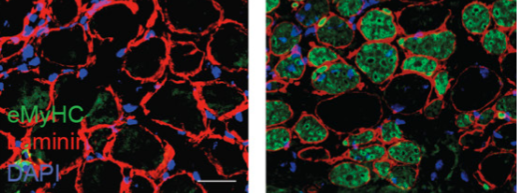